Exact compiled draft

This embedded English PDF is the authoritative layout. It contains the complete AASTeX text, all four tables, all three figures, and the full reference list.

Complete bilingual HTML article

Switch between the exact English manuscript text and a structure-matched academic Chinese translation. Equations, citations, tables, and links are preserved.

Language applies to the HTML article and interface. The compiled PDF and bibliography titles remain in their authoritative English form.

Abstract

The soft X-ray emission toward the inner halo of M31 contains contributions from both M31 and the Milky Way, whose thermal spectra are nearly degenerate at CCD resolution. We analyze 22 XMM-Newton pointings at projected radii of approximately 10–31 kpc and treat the directly measured cool component as the full line-of-sight sum rather than assigning it to either galaxy. Our homogeneous baseline excludes the MOS 1.4–2.0 keV instrumental-line interval, uses a pointing-dependent 15 arcmin HI4PI atomic hydrogen column, and retains 14 technically valid dual-MOS fields in the primary sample. The primary spectra are consistent with a common temperature of \(kT=0.17531\pm0.00436\,\mathrm{keV}\), with no evidence for additional temperature scatter. The absorbed 0.4–1.25 keV surface flux is \((1.106\pm0.054)\,10^{-15}\,\mathrm{erg\,cm^{-2}\,s^{-1}\,arcmin^{-2}}\) in the North/NW fields and \((0.894\pm0.203)\,10^{-15}\,\mathrm{erg\,cm^{-2}\,s^{-1}\,arcmin^{-2}}\) in the South/SE fields. Their difference, \((0.212\pm0.210)\,10^{-15}\,\mathrm{erg\,cm^{-2}\,s^{-1}\,arcmin^{-2}}\), is positive but not statistically compelling. The current data therefore establish a spatially widespread, approximately 0.18 keV line-of-sight component but do not detect a large-scale North–South asymmetry or uniquely identify an M31 contribution. Any decomposition into M31, Milky Way, or Local-Group emission requires an explicit spatial or foreground prior.

Keywords: Andromeda Galaxy; circumgalactic medium; diffuse X-ray background; X-ray astronomy; Milky Way Galaxy

Internal Draft Status

This manuscript is a complete internal scientific draft based on the validated v19 independent-fit baseline. It is not yet ready for submission. The numerical values quoted below use local LevMar covariance matrices. The submission version must replace the descriptive side means with a shared radial model plus a side offset, compute profile-likelihood or simulation-calibrated intervals at non-negative boundaries, and add a controlled spectral-systematic grid. These requirements are summarized in Section 7.

Introduction

Hot circumgalactic gas is expected to contain a substantial fraction of the baryons associated with massive spiral galaxies, but its low density makes direct X-ray measurements difficult. Deep observations of individual massive spirals and stacked samples demonstrate extended soft X-ray halos, while also showing that inferred profiles depend on galaxy mass, unresolved-source subtraction, and background treatment (Anderson et al. 2016; Li et al. 2017, 2018; Zhang, Comparat, Ponti, Merloni, Nandra, Haberl, Locatelli, et al. 2024; Zhang, Comparat, Ponti, Merloni, Nandra, Haberl, Truong, et al. 2024). M31 is close enough that its inner halo can be sampled with multiple XMM-Newton fields, but its large angular extent creates a different limitation: emission from the M31 halo is superposed on spatially structured soft emission from the Milky Way and potentially the Local Group.

The central few kiloparsecs of M31 contain multiphase diffuse X-ray emission associated with the bulge and disk (Shirey et al. 2001; Takahashi et al. 2004; Li and Wang 2007). Those measurements do not determine the amplitude of cooler gas at projected radii of 10–31 kpc. Off-disc XMM-Newton observations provide a closer spectral precedent. Kavanagh et al. (2020) measured a component near \(0.17\)–\(0.18\,\mathrm{keV}\) and explicitly modeled it as the combined emission of the Galaxy, M31, and the intergalactic medium. A possible Local Hot Bridge in the direction of M31 has a similar inferred temperature (Qu et al. 2021). Milky Way surveys also find characteristic temperatures near \(0.15\)–\(0.22\,\mathrm{keV}\) but substantial spatial variation (Henley and Shelton 2013a, 2015; Ponti et al. 2023; Kaaret et al. 2020; Ueda et al. 2022; Locatelli et al. 2024).

These overlapping temperature scales make distance attribution from an EPIC spectrum alone unreliable. We therefore organize the analysis around the directly observed line-of-sight component, \[\begin{equation} S_{\rm obs}(E)=S_{\rm MW}(E)+S_{\rm M31}(E), \label{eq:direct-sum} \end{equation}\] with an optional third Local-Group term in explicitly labeled conditional scenarios. We ask two assumption-light questions. First, what cool thermal surface flux is measured toward the North/NW and South/SE inner-halo fields? Second, how strongly do the data constrain a difference between the two sampled sides? The M31-versus-Milky-Way decomposition is discussed only after these direct measurements.

Observations and Data Reduction

XMM-Newton program and field selection

We use observations from XMM-Newton proposal 080073, “XMM-Newton Legacy Survey of M31 Halo: Searching for the Missing Accreted Hot CGM” (PI J.-T. Li), obtained with the EPIC cameras (Jansen et al. 2001; Turner et al. 2001). The selected observations were taken between 2017 June 28 and 2018 January 17. All 43 detector products used here have the Thin1 optical blocking filter. The v19 analysis is MOS-only: 21 fields have one MOS1 and one MOS2 spectrum, while 0800730101 contributes MOS2 only.

EPIC-pn products are not used in this homogeneous baseline because the retained preliminary pn branch does not provide an equivalently validated particle-background set. In the audited PATTERN<=4 pn branch of the local SAS 20.0.0 reduction, all 22 fields have a source spectrum, but only 21 have a matched QPB spectrum in the same processing branch (the 22nd, 0800730101, has a paired source and QPB in a neighboring PATTERN<=0 branch but not in this one, so “matched” is defined within the same event-selection and processing branch), and 17 of the 22 source PHA files record a cleaned exposure shorter than 10 ks. This is the regime in which the current XMM-ESAS Cookbook identifies a specific pn limitation, known as “The Corner Problem”: the small out-of-field-of-view corner sample has poor counting statistics, is affected by out-of-time events, and is more sensitive than previously recognized to residual Soft Proton flares, so the inferred pn QPB can be under- or over-estimated, including possible oversubtraction (XMM-Newton Science Analysis Centre 2025). We therefore defer pn inclusion until those spectra and their corner-normalized QPB products are reprocessed and validated independently across the full sample. This is a product-level background-systematics choice for the local SAS 20.0.0 pn branch, not a claim that EPIC-pn data are generally unusable or that all current SAS 22.0 pn products share this limitation. The per-field audit is provided in m31_cgmsum_v19_pn_qpb_readiness.csv.

The 22-field parent set is the proposal-080073 subset for which the upstream project screening retained the required diffuse-field products. Observation 0800731701 is absent from the local reduction tree, 0800732401 lacks the required 4.background products, and 0800731201, 0800731401, 0800731801, 0800732501, 0800732901, and 0800733001 were rejected upstream because of extreme 2.0–3.2 keV observed-to-QPB ratios. Observation 0800733101 was rejected because of extreme residual Soft Proton contamination and incomplete MOS coverage. These exclusions define the parent set before the v19 spectral-quality cuts described in Section 4.4; they are not selected on fitted \(\mathrm{CGM}_{\mathrm{sum}}\) temperature or surface flux.

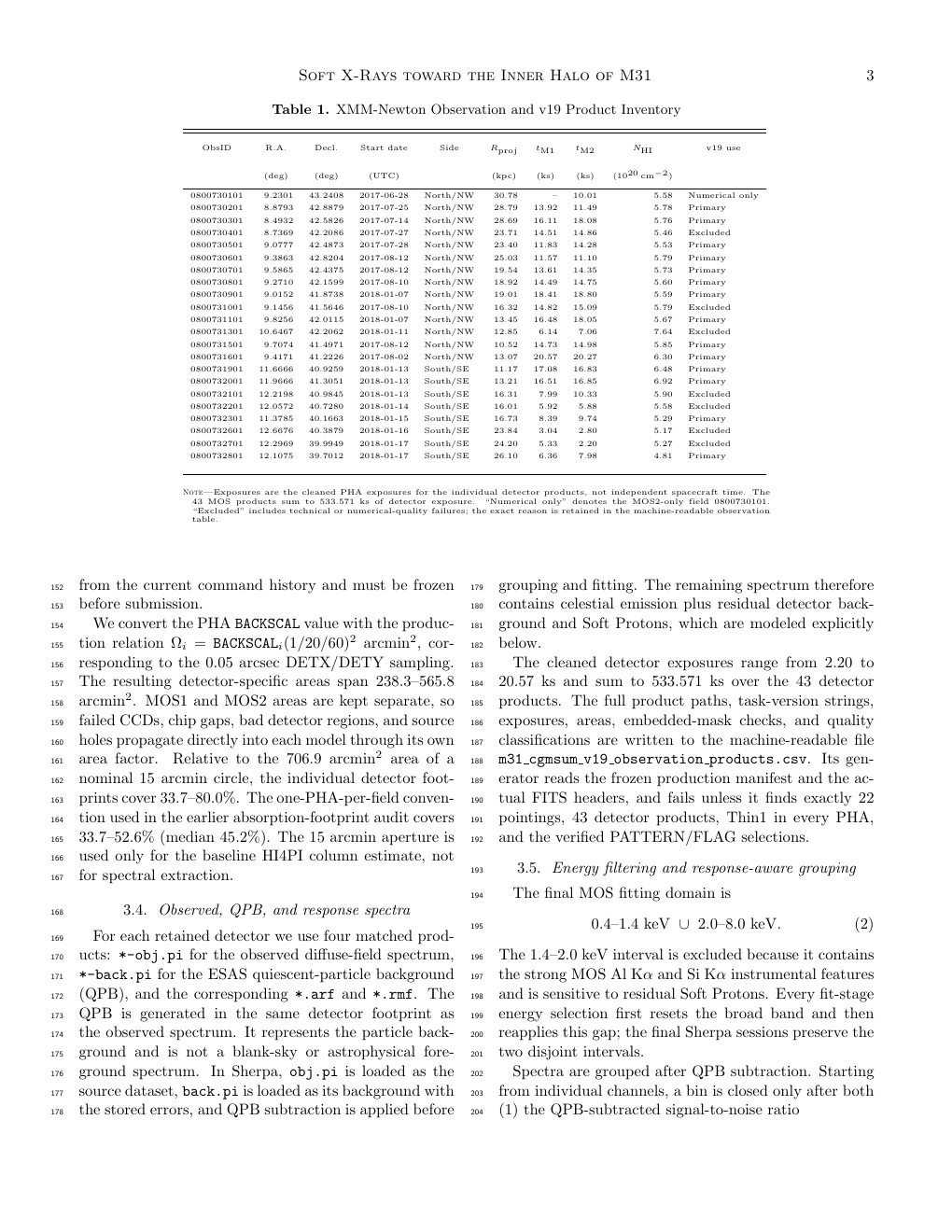
Pointing centers are taken from the final PHA headers. For an adopted M31 center and distance of 785 kpc (McConnachie et al. 2005), their circular projected radii span 10.5–30.8 kpc. The pointings form two approximately minor-axis chains, labeled North/NW and South/SE, rather than a complete azimuthal annulus. In the final primary sample, the median radii are 19.28 and 14.97 kpc on the two sides, respectively, and no South/SE primary field lies at 20–25 kpc. Table 1 gives the observation-level inventory.

Table 1. XMM-Newton Observation and v19 Product Inventory

ObsID	R.A. (deg)	Decl. (deg)	Start date (UTC)	Side	Rproj (kpc)	MOS1 (ks)	MOS2 (ks)	NHI (10²⁰ cm⁻²)	v19 use
0800730101	9.2301	43.2408	2017-06-28	North/NW	30.78	–	10.01	5.58	Numerical only
0800730201	8.8793	42.8879	2017-07-25	North/NW	28.79	13.92	11.49	5.78	Primary
0800730301	8.4932	42.5826	2017-07-14	North/NW	28.69	16.11	18.08	5.76	Primary
0800730401	8.7369	42.2086	2017-07-27	North/NW	23.71	14.51	14.86	5.46	Excluded
0800730501	9.0777	42.4873	2017-07-28	North/NW	23.40	11.83	14.28	5.53	Primary
0800730601	9.3863	42.8204	2017-08-12	North/NW	25.03	11.57	11.10	5.79	Primary
0800730701	9.5865	42.4375	2017-08-12	North/NW	19.54	13.61	14.35	5.73	Primary
0800730801	9.2710	42.1599	2017-08-10	North/NW	18.92	14.49	14.75	5.60	Primary
0800730901	9.0152	41.8738	2018-01-07	North/NW	19.01	18.41	18.80	5.59	Primary
0800731001	9.1456	41.5646	2017-08-10	North/NW	16.32	14.82	15.09	5.79	Excluded
0800731101	9.8256	42.0115	2018-01-07	North/NW	13.45	16.48	18.05	5.67	Primary
0800731301	10.6467	42.2062	2018-01-11	North/NW	12.85	6.14	7.06	7.64	Excluded
0800731501	9.7074	41.4971	2017-08-12	North/NW	10.52	14.73	14.98	5.85	Primary
0800731601	9.4171	41.2226	2017-08-02	North/NW	13.07	20.57	20.27	6.30	Primary
0800731901	11.6666	40.9259	2018-01-13	South/SE	11.17	17.08	16.83	6.48	Primary
0800732001	11.9666	41.3051	2018-01-13	South/SE	13.21	16.51	16.85	6.92	Primary
0800732101	12.2198	40.9845	2018-01-13	South/SE	16.31	7.99	10.33	5.90	Excluded
0800732201	12.0572	40.7280	2018-01-14	South/SE	16.01	5.92	5.88	5.58	Excluded
0800732301	11.3785	40.1663	2018-01-15	South/SE	16.73	8.39	9.74	5.29	Primary
0800732601	12.6676	40.3879	2018-01-16	South/SE	23.84	3.04	2.80	5.17	Excluded
0800732701	12.2969	39.9949	2018-01-17	South/SE	24.20	5.33	2.20	5.27	Excluded
0800732801	12.1075	39.7012	2018-01-17	South/SE	26.10	6.36	7.98	4.81	Primary

Exposures are cleaned PHA detector exposures, not independent spacecraft time. The 43 MOS products sum to 533.571 ks. “Numerical only” is the MOS2-only field 0800730101; excluded fields fail technical or numerical-quality requirements.

SAS processing provenance

The spectra were derived from the existing project reduction with the XMM-Newton Science Analysis System (SAS; Gabriel et al. (2004)). We audited the headers of every v19 input rather than assigning generic “standard SAS” settings. All 43 source PHA files report xmmsas_20211130_0941-20.0.0, evselect-3.71.1; their ARFs report arfgen-1.102.1, and their RMFs report rmfgen-2.8.5. The event selections stored in every PHA require PATTERN<=12 and FLAG==0. The spectra therefore include valid MOS single–quadruple events and reject flagged events.

The final PHAs contain the applied good-time intervals as embedded GTI extensions, but the local tree does not retain the upstream flare-light-curve thresholds or a command log that uniquely reconstructs those GTIs for the full sample. One partial command record survives for 0800732701, but it cannot define a homogeneous 22-field prescription. Likewise, the local ccf.cif files are not bound to the PHA/ARF/RMF products by a recorded identifier or hash, and their file dates do not uniquely establish which calibration index was active during each extraction. We therefore report the verified SAS task versions and final cleaned exposures, but do not invent sample-wide flare thresholds or a CCF release.

The retained tree is sufficient to reproduce the paper analysis from the 43 final spectral product groups. It is not sufficient for a bitwise ODF-to-PHA rebuild: complete ODF material is retained locally for only three selected observations, and original mos-spectra/QPB command files are absent for most fields. Recovery of the homogeneous flare-screening, calibration-index, and extraction-command provenance remains a submission requirement.

Source masks and extraction footprint

The analysis uses the products under rpc/4.background/bkg_mos[12]_00500-02000_exclude_extent_source_mask. The extraction is the usable MOS field of view after detector-coordinate chip/gap masks and point/extended-source exclusions; it is not a simple 15 arcmin circle. The authoritative mask geometry is embedded in each PHA as REGION extensions and in the SLCTEXPR selection. The embedded regions contain negative detector-coordinate ellipses for excluded sources together with the valid chip and field-of-view geometry. The reduction tree also retains the associated edetect_stack source-position and extended-source region products. The exact source-detection likelihood threshold and the rule that maps detections to exclusion-ellipse size are not recoverable from the current command history and must be frozen before submission.

We convert the PHA BACKSCAL value with the production relation \(\Omega_i=\texttt{BACKSCAL}_i(1/20/60)^2\) arcmin\(^2\), corresponding to the 0.05 arcsec DETX/DETY sampling. The resulting detector-specific areas span 238.3–565.8 arcmin\(^2\). MOS1 and MOS2 areas are kept separate, so failed CCDs, chip gaps, bad detector regions, and source holes propagate directly into each model through its own area factor. Relative to the 706.9 arcmin\(^2\) area of a nominal 15 arcmin circle, the individual detector footprints cover 33.7–80.0%. The one-PHA-per-field convention used in the earlier absorption-footprint audit covers 33.7–52.6% (median 45.2%). The 15 arcmin aperture is used only for the baseline HI4PI column estimate, not for spectral extraction.

Observed, QPB, and response spectra

For each retained detector we use four matched products: *-obj.pi for the observed diffuse-field spectrum, *-back.pi for the ESAS quiescent-particle background (QPB), and the corresponding *.arf and *.rmf. The QPB is generated in the same detector footprint as the observed spectrum. It represents the particle background and is not a blank-sky or astrophysical foreground spectrum. In Sherpa, obj.pi is loaded as the source dataset, back.pi is loaded as its background with the stored errors, and QPB subtraction is applied before grouping and fitting. The remaining spectrum therefore contains celestial emission plus residual detector background and Soft Protons, which are modeled explicitly below.

The cleaned detector exposures range from 2.20 to 20.57 ks and sum to 533.571 ks over the 43 detector products. The full product paths, task-version strings, exposures, areas, embedded-mask checks, and quality classifications are written to the machine-readable file m31_cgmsum_v19_observation_products.csv. Its generator reads the frozen production manifest and the actual FITS headers, and fails unless it finds exactly 22 pointings, 43 detector products, Thin1 in every PHA, and the verified PATTERN/FLAG selections.

Energy filtering and response-aware grouping

The final MOS fitting domain is \[\begin{equation} 0.4\text{--}1.4~\mathrm{keV}\ \cup\ 2.0\text{--}8.0~\mathrm{keV}. \label{eq:fitband} \end{equation}\] The 1.4–2.0 keV interval is excluded because it contains the strong MOS Al K\(\alpha\) and Si K\(\alpha\) instrumental features and is sensitive to residual Soft Protons. Every fit-stage energy selection first resets the broad band and then reapplies this gap; the final Sherpa sessions preserve the two disjoint intervals.

Spectra are grouped after QPB subtraction. Starting from individual channels, a bin is closed only after both (1) the QPB-subtracted signal-to-noise ratio \[\begin{equation} {\rm S/N}=\frac{C_{\rm obj}-C_{\rm QPB}} {\sqrt{C_{\rm obj}+C_{\rm QPB}}} \end{equation}\] reaches 6 and (2) its channel width samples the local RMF FWHM by no more than a factor of 6. Group accumulation is reset at ignored channels, and group starts are forced at 0.4, 1.4, 2.0, and 8.0 keV. Consequently, no fitted bin bridges the excluded MOS interval.

Spectral Analysis

Response construction and model topology

We fit each pointing independently in Sherpa 4.18 (Freeman et al. 2001) using XSPEC model components (Arnaud 1996). Within one pointing, the MOS1 and MOS2 celestial parameters are linked, whereas the residual instrumental-line and Soft Proton parameters remain detector specific. No parameter is linked between different pointings. If \(R_i\) denotes the detector RMF folded with its ARF, \(D_i\) denotes the same redistribution with a unit effective area, and \(\Omega_i\) is the PHA solid angle, the count model for detector \(i\) is \[\begin{equation} \begin{split} M_i(E)={}&R_i\Big\{\Omega_i\big[G_i(E)+S_{\rm LB}(E)+S_{\rm SWCX}(E)\\ &+A(N_{{\rm HI},i})\{S_{\rm CXB}(E)+S_{\mathrm{CGM}_{\mathrm{sum}}}(E)\\ &\qquad\qquad\quad+S_{\rm hot}(E)\}\big]\Big\}\\ &+D_i\{\Omega_i P_i(E)\}. \end{split} \label{eq:model} \end{equation}\] Here \(G_i\) is the residual detector-line model, \(P_i\) is the Soft Proton continuum, and the remaining terms are sky surface-brightness components. Multiplication by \(\Omega_i\) converts every surface-brightness normalization to the actual detector footprint before response folding. The multiplicative sky-background scale present in the implementation is fixed to unity.

The component called MWhalo in the fitting code is denoted \(\mathrm{CGM}_{\mathrm{sum}}\) here. It is the cool absorbed APEC component required by the line of sight, not a spectroscopic assignment to the Milky Way. The historical target-specific SrcApec, SrcPo, and Srcabs components remain in the implementation for compatibility but are set to zero and frozen in this independent diffuse-field analysis. Thus no additional M31-only spectral component is fitted on top of \(\mathrm{CGM}_{\mathrm{sum}}\).

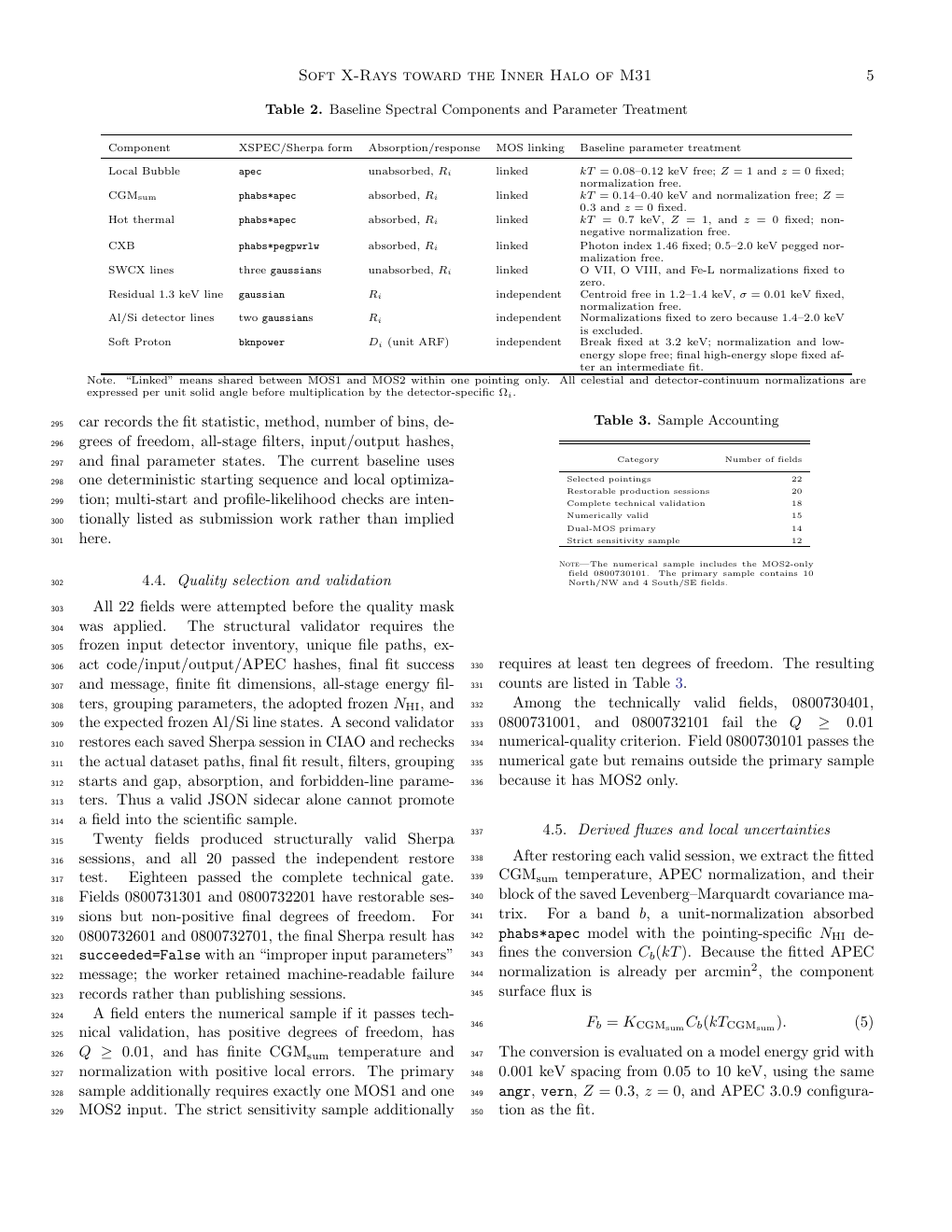
Table 2. Baseline Spectral Components and Parameter Treatment

Component	XSPEC/Sherpa form	Absorption/response	MOS linking	Baseline parameter treatment
Local Bubble	`apec`	unabsorbed, \(R_i\)	linked	\(kT=0.08\)–0.12 keV free; \(Z=1\) and \(z=0\) fixed; normalization free.
\(\mathrm{CGM}_{\mathrm{sum}}\)	`phabs*apec`	absorbed, \(R_i\)	linked	\(kT=0.14\)–0.40 keV and normalization free; \(Z=0.3\) and \(z=0\) fixed.
Hot thermal	`phabs*apec`	absorbed, \(R_i\)	linked	\(kT=0.7\) keV, \(Z=1\), and \(z=0\) fixed; non-negative normalization free.
CXB	`phabs*pegpwrlw`	absorbed, \(R_i\)	linked	Photon index 1.46 fixed; 0.5–2.0 keV pegged normalization free.
SWCX lines	three `gaussian`s	unabsorbed, \(R_i\)	linked	O VII, O VIII, and Fe-L normalizations fixed to zero.
Residual 1.3 keV line	`gaussian`	\(R_i\)	independent	Centroid free in 1.2–1.4 keV, \(\sigma=0.01\) keV fixed, normalization free.
Al/Si detector lines	two `gaussian`s	\(R_i\)	independent	Normalizations fixed to zero because 1.4–2.0 keV is excluded.
Soft Proton	`bknpower`	\(D_i\) (unit ARF)	independent	Break fixed at 3.2 keV; normalization and low-energy slope free; final high-energy slope fixed after an intermediate fit.

Note. “Linked” means shared between MOS1 and MOS2 within one pointing only. All celestial and detector-continuum normalizations are expressed per unit solid angle before multiplication by the detector-specific \(\Omega_i\).

Ri denotes the full ARF/RMF response; Di denotes the RMF plus unit-ARF response used for residual Soft Protons.

Absorption and atomic configuration

For each pointing, the absorption column is fixed to the uniform-area mean of the HI4PI atomic \(N_{\rm HI}\) map within a 15 arcmin aperture (HI4PI Collaboration 2016). The adopted values span \(4.81\times10^{20}\) to \(7.65\times10^{20}\,\mathrm{cm^{-2}}\). The map has a native angular resolution of 16.2 arcmin; a nominal aperture therefore contains only about 2.38 independent beams. The aperture is centered on the pointing coordinate, has complete valid-map coverage, and is not weighted by the MOS source mask or exposure map.

These inputs are atomic H I columns, not total equivalent X-ray absorbing columns. Molecular gas, dust-to-gas conversion, 21-cm optical-depth corrections, and the mismatch between the circular HI4PI aperture and the irregular MOS footprints are not included in the formal errors. They are retained as controlled absorption-systematics branches.

The XSPEC configuration is fixed to the angr solar-abundance table, vern photoelectric cross sections, and APEC/AtomDB 3.0.9 (Foster et al. 2012). The exact APEC line and continuum files are present in the CIAO installation and their SHA-256 hashes are stored in the production manifest.

Staged fitting procedure

All fits use the Gehrels chi-square statistic (chi2gehrels) and the Sherpa Levenberg–Marquardt optimizer. The staged procedure is identical for every pointing:

In the initial \(0.2\)–\(1.4\cup2.0\)–\(8.0\) keV fit, set the Local Bubble to \(kT=0.1\) keV and \(Z=1\), set \(\mathrm{CGM}_{\mathrm{sum}}\) to \(kT=0.2\) keV and \(Z=0.3\), and fix the hot component to \(kT=0.7\) keV and \(Z=1\). The Local Bubble, \(\mathrm{CGM}_{\mathrm{sum}}\), hot-component, and CXB normalizations are free. The per-detector Soft Proton normalization and both slopes are initially frozen with zero normalization. The three SWCX line normalizations remain zero.
Thaw the Local Bubble and \(\mathrm{CGM}_{\mathrm{sum}}\) temperatures within the bounds in Table 2, keep both abundances fixed, and refit the linked MOS spectra.
Apply the final domain in Equation 2 and refit the thermal, CXB, and residual-line parameters.
For each detector, thaw the broken-power-law normalization and both photon indices while keeping the 3.2 keV break fixed, and refit all active parameters jointly.
Freeze the fitted high-energy Soft Proton index. Refit the low-energy index and normalization with the physical ordering \(0\leq\Gamma_{\rm low}\leq\Gamma_{\rm high}\); if the unconstrained intermediate fit violates the ordering, initialize \(\Gamma_{\rm low}=\Gamma_{\rm high}/2\) before the final fit.

The production worker publishes a session only when Sherpa reports succeeded=True. Every published sidecar records the fit statistic, method, number of bins, degrees of freedom, all-stage filters, input/output hashes, and final parameter states. The current baseline uses one deterministic starting sequence and local optimization; multi-start and profile-likelihood checks are intentionally listed as submission work rather than implied here.

Quality selection and validation

All 22 fields were attempted before the quality mask was applied. The structural validator requires the frozen input detector inventory, unique file paths, exact code/input/output/APEC hashes, final fit success and message, finite fit dimensions, all-stage energy filters, grouping parameters, the adopted frozen \(N_{\rm HI}\), and the expected frozen Al/Si line states. A second validator restores each saved Sherpa session in CIAO and rechecks the actual dataset paths, final fit result, filters, grouping starts and gap, absorption, and forbidden-line parameters. Thus a valid JSON sidecar alone cannot promote a field into the scientific sample.

Twenty fields produced structurally valid Sherpa sessions, and all 20 passed the independent restore test. Eighteen passed the complete technical gate. Fields 0800731301 and 0800732201 have restorable sessions but non-positive final degrees of freedom. For 0800732601 and 0800732701, the final Sherpa result has succeeded=False with an “improper input parameters” message; the worker retained machine-readable failure records rather than publishing sessions.

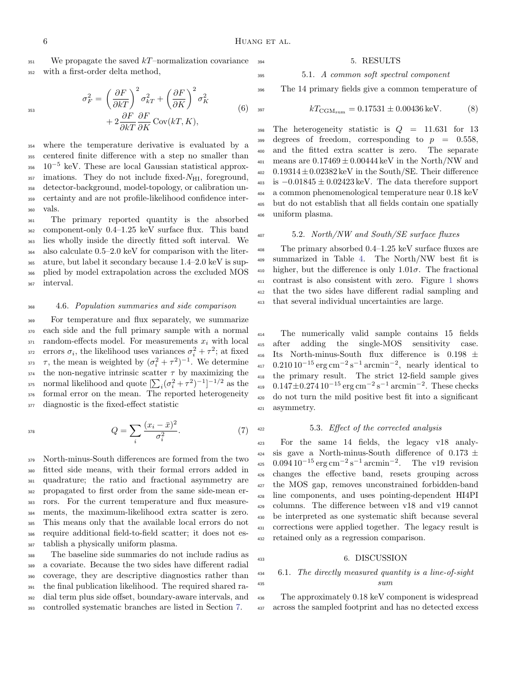
A field enters the numerical sample if it passes technical validation, has positive degrees of freedom, has \(Q\geq0.01\), and has finite \(\mathrm{CGM}_{\mathrm{sum}}\) temperature and normalization with positive local errors. The primary sample additionally requires exactly one MOS1 and one MOS2 input. The strict sensitivity sample additionally requires at least ten degrees of freedom. The resulting counts are listed in Table 3.

Among the technically valid fields, 0800730401, 0800731001, and 0800732101 fail the \(Q\geq0.01\) numerical-quality criterion. Field 0800730101 passes the numerical gate but remains outside the primary sample because it has MOS2 only.

Table 3. Sample Accounting

Category	Number of fields
Selected pointings	22
Restorable production sessions	20
Complete technical validation	18
Numerically valid	15
Dual-MOS primary	14
Strict sensitivity sample	12

The numerical sample includes MOS2-only 0800730101. The primary sample contains 10 North/NW and 4 South/SE fields.

Derived fluxes and local uncertainties

After restoring each valid session, we extract the fitted \(\mathrm{CGM}_{\mathrm{sum}}\) temperature, APEC normalization, and their block of the saved Levenberg–Marquardt covariance matrix. For a band \(b\), a unit-normalization absorbed phabs*apec model with the pointing-specific \(N_{\rm HI}\) defines the conversion \(C_b(kT)\). Because the fitted APEC normalization is already per arcmin\(^2\), the component surface flux is \[\begin{equation} F_b=K_{\mathrm{CGM}_{\mathrm{sum}}}C_b(kT_{\mathrm{CGM}_{\mathrm{sum}}}). \end{equation}\] The conversion is evaluated on a model energy grid with 0.001 keV spacing from 0.05 to 10 keV, using the same angr, vern, \(Z=0.3\), \(z=0\), and APEC 3.0.9 configuration as the fit.

We propagate the saved \(kT\)–normalization covariance with a first-order delta method, \[\begin{equation} \begin{split} \sigma_F^2={}&\left(\frac{\partial F}{\partial kT}\right)^2\sigma_{kT}^2+ \left(\frac{\partial F}{\partial K}\right)^2\sigma_K^2\\ &+2\frac{\partial F}{\partial kT}\frac{\partial F}{\partial K}\, \mathrm{Cov}(kT,K), \end{split} \end{equation}\] where the temperature derivative is evaluated by a centered finite difference with a step no smaller than \(10^{-5}\) keV. These are local Gaussian statistical approximations. They do not include fixed-\(N_{\rm HI}\), foreground, detector-background, model-topology, or calibration uncertainty and are not profile-likelihood confidence intervals.

The primary reported quantity is the absorbed component-only 0.4–1.25 keV surface flux. This band lies wholly inside the directly fitted soft interval. We also calculate 0.5–2.0 keV for comparison with the literature, but label it secondary because 1.4–2.0 keV is supplied by model extrapolation across the excluded MOS interval.

Population summaries and side comparison

For temperature and flux separately, we summarize each side and the full primary sample with a normal random-effects model. For measurements \(x_i\) with local errors \(\sigma_i\), the likelihood uses variances \(\sigma_i^2+\tau^2\); at fixed \(\tau\), the mean is weighted by \((\sigma_i^2+\tau^2)^{-1}\). We determine the non-negative intrinsic scatter \(\tau\) by maximizing the normal likelihood and quote \([\sum_i(\sigma_i^2+\tau^2)^{-1}]^{-1/2}\) as the formal error on the mean. The reported heterogeneity diagnostic is the fixed-effect statistic \[\begin{equation} Q=\sum_i \frac{(x_i-\bar{x})^2}{\sigma_i^2}. \end{equation}\] North-minus-South differences are formed from the two fitted side means, with their formal errors added in quadrature; the ratio and fractional asymmetry are propagated to first order from the same side-mean errors. For the current temperature and flux measurements, the maximum-likelihood extra scatter is zero. This means only that the available local errors do not require additional field-to-field scatter; it does not establish a physically uniform plasma.

The baseline side summaries do not include radius as a covariate. Because the two sides have different radial coverage, they are descriptive diagnostics rather than the final publication likelihood. The required shared radial term plus side offset, boundary-aware intervals, and controlled systematic branches are listed in Section 7.

Results

A common soft spectral component

The 14 primary fields give a common temperature of \[\begin{equation} kT_{\mathrm{CGM}_{\mathrm{sum}}}=0.17531\pm0.00436\,\mathrm{keV}. \end{equation}\] The heterogeneity statistic is \(Q=11.631\) for 13 degrees of freedom, corresponding to \(p=0.558\), and the fitted extra scatter is zero. The separate means are \(0.17469\pm0.00444\,\mathrm{keV}\) in the North/NW and \(0.19314\pm0.02382\,\mathrm{keV}\) in the South/SE. Their difference is \(-0.01845\pm0.02423\,\mathrm{keV}\). The data therefore support a common phenomenological temperature near 0.18 keV but do not establish that all fields contain one spatially uniform plasma.

North/NW and South/SE surface fluxes

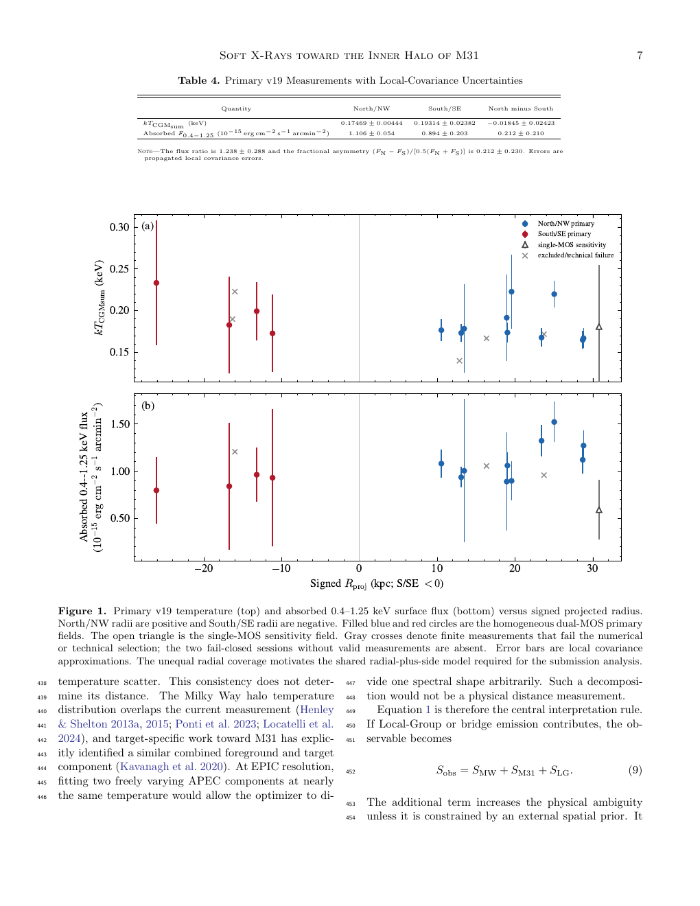
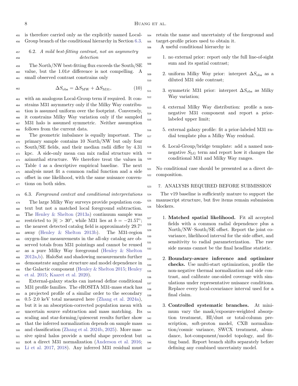
The primary absorbed 0.4–1.25 keV surface fluxes are summarized in Table 4. The North/NW best fit is higher, but the difference is only \(1.01\sigma\). The fractional contrast is also consistent with zero. Figure 1 shows that the two sides have different radial sampling and that several individual uncertainties are large.

Table 4. Primary v19 Measurements with Local-Covariance Uncertainties

Quantity	North/NW	South/SE	North minus South
kT_CGMsum (keV)	0.17469 ± 0.00444	0.19314 ± 0.02382	−0.01845 ± 0.02423
Absorbed F_0.4–1.25 (10⁻¹⁵ erg cm⁻² s⁻¹ arcmin⁻²)	1.106 ± 0.054	0.894 ± 0.203	0.212 ± 0.210

The flux ratio is 1.238 ± 0.288 and the fractional asymmetry is 0.212 ± 0.230. Errors are propagated local-covariance errors, not profile-likelihood intervals.

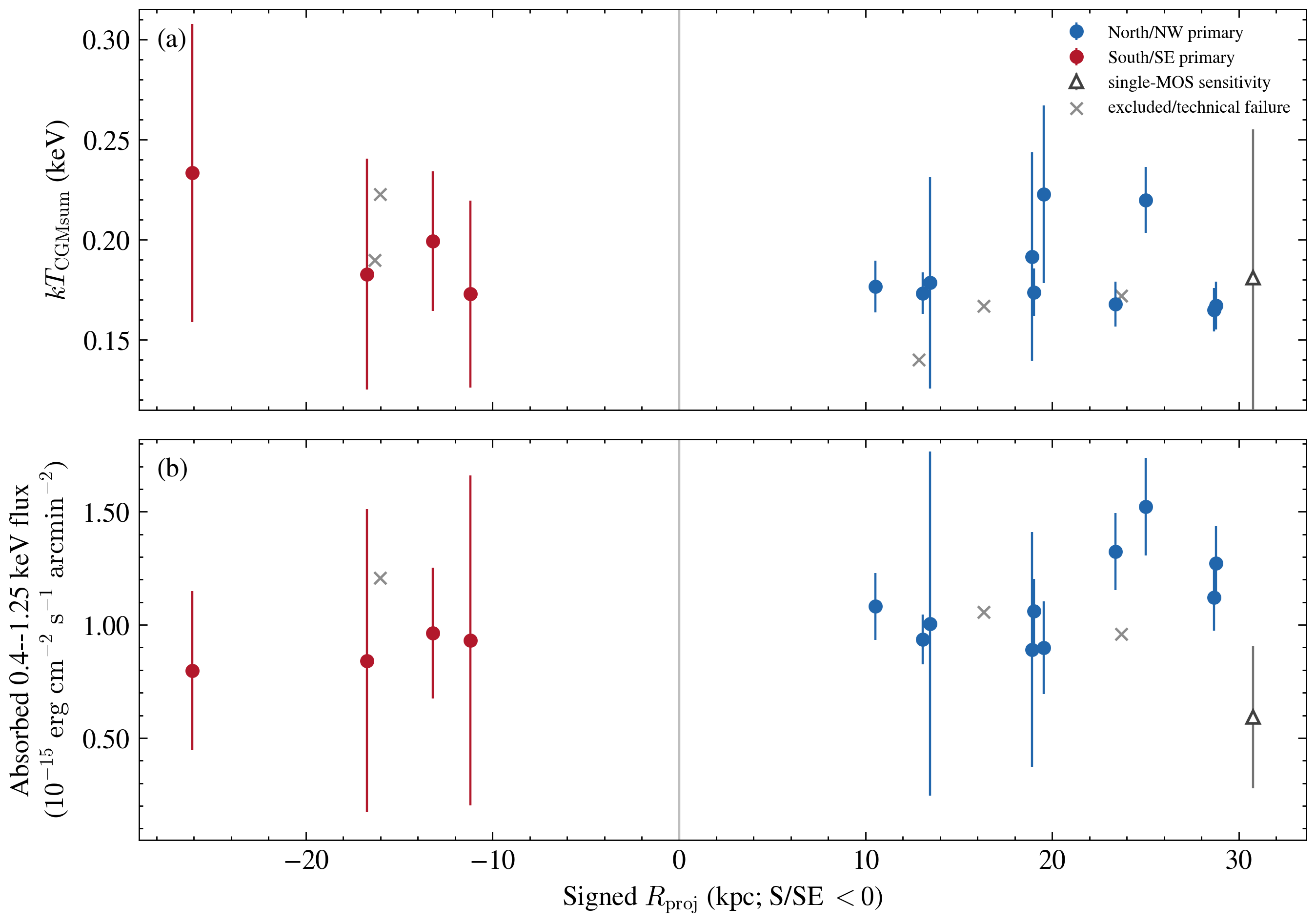
CGMsum temperature and absorbed 0.4–1.25 keV surface flux versus signed projected radius — Primary v19 temperature (top) and absorbed 0.4–1.25 keV surface flux (bottom) versus signed projected radius. North/NW radii are positive and South/SE radii are negative. Filled blue and red circles are the homogeneous dual-MOS primary fields. The open triangle is the single-MOS sensitivity field. Gray crosses denote finite measurements that fail the numerical or technical selection; the two fail-closed sessions without valid measurements are absent. Error bars are local covariance approximations. The unequal radial coverage motivates the shared radial-plus-side model required for the submission analysis.

The numerically valid sample contains 15 fields after adding the single-MOS sensitivity case. Its North-minus-South flux difference is \(0.198\pm0.210\,10^{-15}\,\mathrm{erg\,cm^{-2}\,s^{-1}\,arcmin^{-2}}\), nearly identical to the primary result. The strict 12-field sample gives \(0.147\pm0.274\,10^{-15}\,\mathrm{erg\,cm^{-2}\,s^{-1}\,arcmin^{-2}}\). These checks do not turn the mild positive best fit into a significant asymmetry.

Effect of the corrected analysis

For the same 14 fields, the legacy v18 analysis gave a North-minus-South difference of \(0.173\pm0.094\,10^{-15}\,\mathrm{erg\,cm^{-2}\,s^{-1}\,arcmin^{-2}}\). The v19 revision changes the effective band, resets grouping across the MOS gap, removes unconstrained forbidden-band line components, and uses pointing-dependent HI4PI columns. The difference between v18 and v19 cannot be interpreted as one systematic shift because several corrections were applied together. The legacy result is retained only as a regression comparison.

Discussion

The directly measured quantity is a line-of-sight sum

The approximately 0.18 keV component is widespread across the sampled footprint and has no detected excess temperature scatter. This consistency does not determine its distance. The Milky Way halo temperature distribution overlaps the current measurement (Henley and Shelton 2013a, 2015; Ponti et al. 2023; Locatelli et al. 2024), and target-specific work toward M31 has explicitly identified a similar combined foreground and target component (Kavanagh et al. 2020). At EPIC resolution, fitting two freely varying APEC components at nearly the same temperature would allow the optimizer to divide one spectral shape arbitrarily. Such a decomposition would not be a physical distance measurement.

Equation 1 is therefore the central interpretation rule. If Local-Group or bridge emission contributes, the observable becomes \[\begin{equation} S_{\rm obs}=S_{\rm MW}+S_{\rm M31}+S_{\rm LG}. \end{equation}\] The additional term increases the physical ambiguity unless it is constrained by an external spatial prior. It is therefore carried only as the explicitly named Local-Group branch of the conditional hierarchy in Section 6.3.

A mild best-fitting contrast, not an asymmetry detection

The North/NW best-fitting flux exceeds the South/SE value, but the \(1.01\sigma\) difference is not compelling. A small observed contrast constrains only \[\begin{equation} \Delta S_{\rm obs}=\Delta S_{\rm MW}+\Delta S_{\rm M31}, \label{eq:contrast} \end{equation}\] with an analogous Local-Group term if required. It constrains M31 asymmetry only if the Milky Way contribution is assumed uniform over the footprint. Conversely, it constrains Milky Way variation only if the sampled M31 halo is assumed symmetric. Neither assumption follows from the current data.

The geometric imbalance is equally important. The primary sample contains 10 North/NW but only four South/SE fields, and their median radii differ by 4.31 kpc. A side-only mean can mix radial structure with azimuthal structure. We therefore treat the values in Table 4 as a descriptive empirical baseline. The next analysis must fit a common radial function and a side offset in one likelihood, with the same nuisance conventions on both sides.

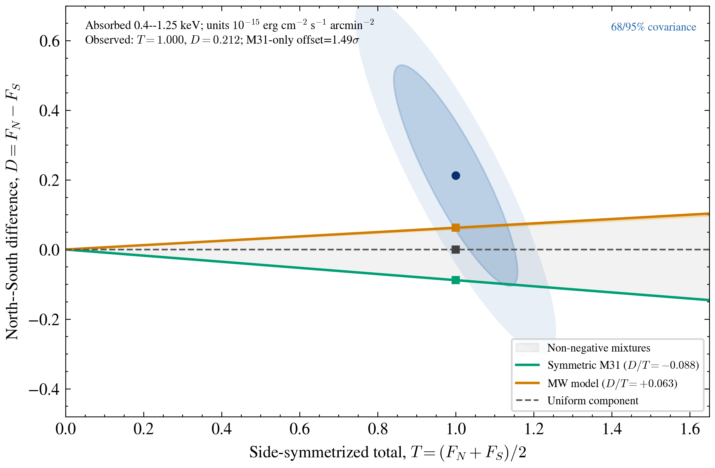
Figure 2 makes the geometric mixing explicit. We define the side-symmetrized total and contrast as \[\begin{equation} T=\frac{F_{\rm N}+F_{\rm S}}{2},\qquad D=F_{\rm N}-F_{\rm S}. \end{equation}\] The primary measurements give \(T=1.000\,10^{-15}\,\mathrm{erg\,cm^{-2}\,s^{-1}\,arcmin^{-2}}\) and \(D=0.212\,10^{-15}\,\mathrm{erg\,cm^{-2}\,s^{-1}\,arcmin^{-2}}\). Because the same two side means enter both quantities, their errors are strongly covariant; the confidence ellipses in Figure 2 use the full linear transformation of the two local-covariance errors rather than independent horizontal and vertical error bars.

Projecting the Zhang, Comparat, Ponti, Merloni, Nandra, Haberl, Locatelli, et al. (2024) symmetric M31-mass beta profile through the actual 14-field estimator gives \(D/T=-0.088\): the inverse-variance-weighted North/NW fields lie at larger M31 radii and are predicted to be slightly fainter. In contrast, the disk-like plus spherical Milky Way models of Locatelli et al. (2024), including the HI4PI absorption variation across the same pointings, give \(D/T=+0.058\) to \(+0.063\) because the North/NW fields lie closer to the Galactic plane. At the observed \(T\), the residuals from a uniform component, the symmetric-M31 template, and the central Milky Way template are \(1.01\sigma\), \(1.49\sigma\), and \(0.69\sigma\), respectively, after propagating the \(T\)–\(D\) covariance. The positive best fit therefore points in the direction expected for a Galactic latitude gradient, but the present uncertainty does not exclude a uniform component, a symmetric M31 profile, or any non-negative mixture between the two template families. Figure 2 is consequently an exploratory geometry diagnostic, not evidence against a Milky Way or M31 spatial model.

Side-symmetrized total versus North-minus-South difference with MW and M31 spatial templates — Conditional prediction plane for the side-symmetrized total \(T\) and North-minus-South difference \(D\), in absorbed 0.4–1.25 keV units. The blue ellipses are the 68 and 95 percent local-covariance regions obtained by transforming the North/NW and South/SE errors. The green ray is the symmetric Zhang, Comparat, Ponti, Merloni, Nandra, Haberl, Locatelli, et al. (2024) M31 beta-profile prediction after projection through the actual primary estimator. The orange ray and narrow band are the central and systematic-family projections of the Locatelli et al. (2024) Milky Way morphology, including pointing-dependent HI4PI absorption. The gray wedge contains non-negative mixtures of these two component shapes. Squares mark each template prediction at the observed \(T\). No template is rejected at a useful significance.

Foreground and M31 priors in a two-component constraint plane

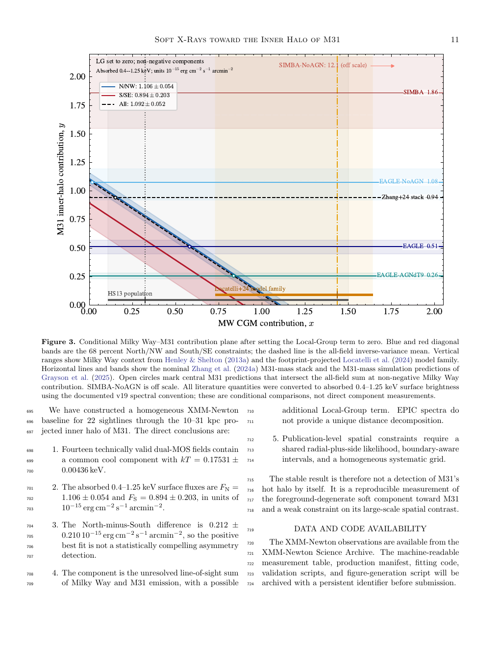
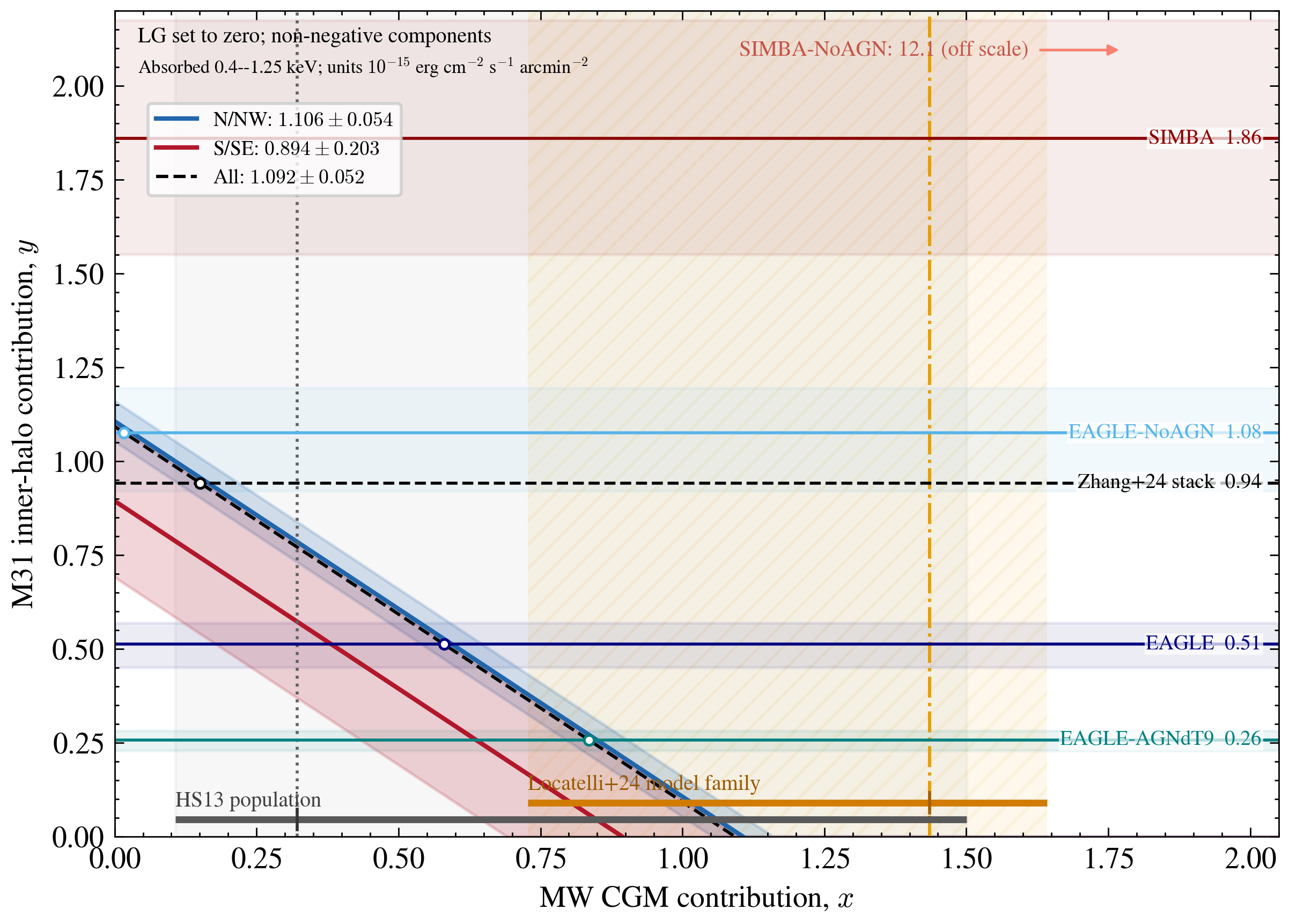
Figure 3 temporarily sets \(S_{\rm LG}=0\) and represents the Milky Way and M31 terms by characteristic footprint-averaged values \(x\) and \(y\). Under this explicit approximation, the North/NW and South/SE measurements become two parallel constraints, \(x+y=1.106\pm0.054\) and \(x+y=0.894\pm0.203\), respectively. Their overlap constrains a sum, not a distance decomposition. Horizontal or vertical literature bands become conditional external priors, and an intersection with a diagonal band is an inference under that named prior rather than an independent measurement of either component.

The Henley and Shelton (2013a) continuum survey supplies the broad gray vertical context in Figure 3. Its intrinsic 0.5–2.0 keV range of \(0.5\)–\(7.0\times10^{-12}\,\mathrm{erg\,cm^{-2}\,s^{-1}\,deg^{-2}}\) and median \(1.5\times10^{-12}\) convert to \(x=0.107\)–\(1.501\,10^{-15}\,\mathrm{erg\,cm^{-2}\,s^{-1}\,arcmin^{-2}}\) and a median \(0.322\,10^{-15}\,\mathrm{erg\,cm^{-2}\,s^{-1}\,arcmin^{-2}}\) for the v19 \(kT=0.175\) keV APEC template. This is deliberately labeled population context: the catalog requires \(|b|>30^\circ\), M31 lies at \(b=-21.57^\circ\), and the nearest detected catalog field is about \(29.7^\circ\) away (Henley and Shelton 2013b). The M31-region oxygen-line catalog entries are observed totals from M31 pointings and are therefore not reused as a pure Milky Way prior (Henley and Shelton 2012a, 2012b).

The orange vertical band is a direction-dependent but more model-dependent alternative. We project the seven disk-like, spherical-plus-disk, SWCX, instrumental-background, and high-emissivity variants tabulated by Locatelli et al. (2024) through the 14 primary sightlines and the same inverse-variance side estimators. Converting their O VIII-fitted density models to the absorbed 0.4–1.25 keV band with each variant’s thermochemistry and the field-specific HI4PI column gives \(x=0.728\)–\(1.642\,10^{-15}\,\mathrm{erg\,cm^{-2}\,s^{-1}\,arcmin^{-2}}\); the combined-plus-SWCX variant gives \(1.435\,10^{-15}\,\mathrm{erg\,cm^{-2}\,s^{-1}\,arcmin^{-2}}\). These values are an interpolation of a three-dimensional O VIII morphology, not a local broadband measurement. Most of the central model family leaves little or no non-negative M31 residual, so the apparent tension tests the adopted O VIII-to-broadband conversion and foreground-screen model at least as much as it tests M31 emission. HaloSat and shadowing measurements independently warn that angular structure and foreground modeling remain important (Henley and Shelton 2015; Henley et al. 2015; Kaaret et al. 2020).

The empirical horizontal reference comes from the M31-stellar-mass eROSITA stack of Zhang, Comparat, Ponti, Merloni, Nandra, Haberl, Locatelli, et al. (2024). Evaluating its nominal beta profile at 20 kpc and converting its intrinsic 0.5–2.0 keV luminosity surface density with the same APEC template gives \(y=0.942\,10^{-15}\,\mathrm{erg\,cm^{-2}\,s^{-1}\,arcmin^{-2}}\). Its intersection with the all-field sum corresponds to a conditional Milky Way residual of \(x\simeq0.151\,10^{-15}\,\mathrm{erg\,cm^{-2}\,s^{-1}\,arcmin^{-2}}\). This line is not a formal prior interval: the published marginalized beta-profile errors lack the covariance required for a reliable 10–30 kpc envelope, and the population stack remains sensitive to mass matching and unresolved-source subtraction. The associated scaling and star-forming/quiescent analyses demonstrate the same normalization dependence (Zhang, Comparat, Ponti, Merloni, Nandra, Haberl, Truong, et al. 2024, 2025).

The simulation predictions in Grayson et al. (2025) span a much larger range. Digitizing their 10–30 kpc M31-mass bin and applying the same band conversion gives \(y=0.257\) for EAGLE-AGNdT9, \(0.512\) for fiducial EAGLE, \(1.076\) for EAGLE-NoAGN, and \(1.859\,10^{-15}\,\mathrm{erg\,cm^{-2}\,s^{-1}\,arcmin^{-2}}\) for fiducial SIMBA; the bootstrap bands are \(0.228\)–\(0.281\), \(0.450\)–\(0.568\), \(0.920\)–\(1.194\), and \(1.549\)–\(2.174\,10^{-15}\,\mathrm{erg\,cm^{-2}\,s^{-1}\,arcmin^{-2}}\), respectively. SIMBA-NoAGN gives \(y=12.13\,10^{-15}\,\mathrm{erg\,cm^{-2}\,s^{-1}\,arcmin^{-2}}\) and is off scale. Under \(x\geq0\), EAGLE-AGNdT9 and fiducial EAGLE require substantial Milky Way residuals, EAGLE-NoAGN lies close to the full observed sum, and both SIMBA predictions exceed it before any Milky Way term is added. This comparison is potentially discriminating, but remains conditional because one v19 APEC spectrum was used to convert intrinsically multiphase simulation emission.

Conditional Milky Way versus M31 contribution plane — Conditional Milky Way–M31 contribution plane after setting the Local-Group term to zero. Blue and red diagonal bands are the 68 percent North/NW and South/SE constraints; the dashed line is the all-field inverse-variance mean. Vertical ranges show Milky Way context from Henley and Shelton (2013a) and the footprint-projected Locatelli et al. (2024) model family. Horizontal lines and bands show the nominal Zhang, Comparat, Ponti, Merloni, Nandra, Haberl, Locatelli, et al. (2024) M31-mass stack and the M31-mass simulation predictions of Grayson et al. (2025). Open circles mark central M31 predictions that intersect the all-field sum at non-negative Milky Way contribution. SIMBA-NoAGN is off scale. All literature quantities were converted to absorbed 0.4–1.25 keV surface brightness using the documented v19 spectral convention; these are conditional comparisons, not direct component measurements.

More massive spiral halos provide useful shape precedents but not a direct M31 normalization (Anderson et al. 2016; Li et al. 2017, 2018). Any inferred M31 residual must retain the name, band conversion, and uncertainty of the foreground and target-profile priors used to obtain it.

A useful conditional hierarchy is:

no external prior: report only the full line-of-sight sum and its spatial contrast;
uniform Milky Way prior: interpret \(\Delta S_{\rm obs}\) as a diluted M31 side contrast;
symmetric M31 prior: interpret \(\Delta S_{\rm obs}\) as Milky Way variation;
external Milky Way distribution: profile a non-negative M31 component and report a prior-labeled upper limit;
external galaxy profile: fit a prior-labeled M31 radial template plus a Milky Way residual.
Local-Group/bridge template: add a named non-negative \(S_{\rm LG}\) term and report how it changes the conditional M31 and Milky Way ranges.

No conditional case should be presented as a direct decomposition.

Analysis Required before Submission

The v19 baseline is sufficiently mature to support the manuscript structure, but five items remain submission blockers.

Matched spatial likelihood. Fit all accepted fields with a common radial dependence plus a North/NW–South/SE offset. Report the joint covariance, likelihood interval for the side offset, and sensitivity to radial parameterization. The raw side means cannot be the final headline statistic.
Boundary-aware inference and optimizer checks. Use multi-start optimization, profile the non-negative thermal normalization and side contrast, and calibrate one-sided coverage with simulations under representative nuisance conditions. Replace every local-covariance interval used for a final claim.
Controlled systematic branches. At minimum vary the mask/exposure-weighted absorption treatment, HI/dust or total-column prescription, soft-proton model, CXB normalization/cosmic variance, SWCX treatment, abundance, hot-component/model topology, and fitting band. Report branch shifts separately before defining any combined uncertainty model.
Quantitative constraint product. Report a calibrated interval on the side offset or fractional asymmetry and at least the conservative U0 upper envelope obtained by assigning the full cool line-of-sight component to M31. A named-prior U1 or smooth-foreground U2 M31 limit would substantially strengthen a full ApJ article, but must remain explicitly conditional.
Submission documentation and figures. Recover the original flare-screening thresholds, bind each extraction to its calibration index, and freeze the source-detection likelihood and mask-radius rule. Add a sky-footprint figure, representative rebinned spectra and residuals, the radial-plus-side fit, and a systematic-branch summary. Archive the current observation table, code, and machine-readable product inventory with persistent versioning.

An absolute M31-versus-Milky-Way decomposition is not a required blocker if the paper remains explicitly about the line-of-sight sum. It becomes a blocker only for claims of a detected M31 halo component or a foreground-subtracted M31 luminosity. A matched off-M31 control field or an external foreground prior would strengthen that second, conditional layer.

Conclusions

We have constructed a homogeneous XMM-Newton baseline for 22 sightlines through the 10–31 kpc projected inner halo of M31. The direct conclusions are:

Fourteen technically valid dual-MOS fields contain a common cool component with \(kT=0.17531\pm0.00436\,\mathrm{keV}\).
The absorbed 0.4–1.25 keV surface fluxes are \(F_{\rm N}=1.106\pm0.054\) and \(F_{\rm S}=0.894\pm0.203\), in units of \(10^{-15}\,\mathrm{erg\,cm^{-2}\,s^{-1}\,arcmin^{-2}}\).
The North-minus-South difference is \(0.212\pm0.210\,10^{-15}\,\mathrm{erg\,cm^{-2}\,s^{-1}\,arcmin^{-2}}\), so the positive best fit is not a statistically compelling asymmetry detection.
The component is the unresolved line-of-sight sum of Milky Way and M31 emission, with a possible additional Local-Group term. EPIC spectra do not provide a unique distance decomposition.
Publication-level spatial constraints require a shared radial-plus-side likelihood, boundary-aware intervals, and a homogeneous systematic grid.

The stable result is therefore not a detection of M31’s hot halo by itself. It is a reproducible measurement of the foreground-degenerate soft component toward M31 and a weak constraint on its large-scale spatial contrast.

Data and Code Availability

The XMM-Newton observations are available from the XMM-Newton Science Archive. The machine-readable measurement table, production manifest, fitting code, validation scripts, and figure-generation script will be archived with a persistent identifier before submission.

This work made use of XMM-Newton data and the HI4PI atomic hydrogen survey. Full acknowledgments, proposal information, and funding statements will be added after the author list is finalized.

References

Anderson, Michael E., Eugene Churazov, and Joel N. Bregman. 2016. “A Deep XMM-Newton Study of the Hot Gaseous Halo Around NGC 1961.” Monthly Notices of the Royal Astronomical Society 455 (1): 227–43. https://doi.org/10.1093/mnras/stv2314.

Arnaud, K. A. 1996. “XSPEC: The First Ten Years.” Astronomical Data Analysis Software and Systems v, Astronomical society of the pacific conference series, vol. 101: 17.

Foster, A. R., L. Ji, R. K. Smith, and N. S. Brickhouse. 2012. “Updated Atomic Data and Calculations for x-Ray Spectroscopy.” The Astrophysical Journal 756: 128. https://doi.org/10.1088/0004-637X/756/2/128.

Freeman, Peter, Stephen Doe, and Aneta Siemiginowska. 2001. “Sherpa: A Mission-Independent Data Analysis Application.” Astronomical Data Analysis, Proceedings of SPIE, vol. 4477: 76–87. https://doi.org/10.1117/12.447161.

Gabriel, C., M. Denby, D. J. Fyfe, et al. 2004. “The XMM-Newton SAS: Distributed Development and Maintenance of a Large Science Analysis System: A Critical Analysis.” Astronomical Data Analysis Software and Systems XIII, Astronomical society of the pacific conference series, vol. 314: 759.

Grayson, Skylar, Evan Scannapieco, Johan Comparat, et al. 2025. “The Hot Circumgalactic Medium in Stacked x-Rays: Observations Versus Simulations.” The Astrophysical Journal 994 (1): 89. https://doi.org/10.3847/1538-4357/ae100f.

Henley, David B., and Robin L. Shelton. 2012a. “An XMM-Newton Survey of the Soft x-Ray Background. II. An All-Sky Catalog of Diffuse o VII and o VIII Emission Intensities.” The Astrophysical Journal Supplement Series 202 (2): 14. https://doi.org/10.1088/0067-0049/202/2/14.

Henley, David B., and Robin L. Shelton. 2012b. VizieR Online Data Catalog: Diffuse o VII and o VIII Emission from XMM. VizieR Online Data Catalog J/ApJS/202/14. https://doi.org/10.26093/cds/vizier.22020014.

Henley, David B., and Robin L. Shelton. 2013a. “An XMM-Newton Survey of the Soft x-Ray Background. III. The Galactic Halo x-Ray Emission.” The Astrophysical Journal 773 (2): 92. https://doi.org/10.1088/0004-637X/773/2/92.

Henley, David B., and Robin L. Shelton. 2013b. VizieR Online Data Catalog: XMM Survey of Soft Background. III. Galactic Halo. VizieR Online Data Catalog J/ApJ/773/92. https://doi.org/10.26093/cds/vizier.17730092.

Henley, David B., and Robin L. Shelton. 2015. “XMM-Newton and Suzaku x-Ray Shadowing Measurements of the Solar Wind Charge Exchange, Local Bubble, and Galactic Halo Emission.” The Astrophysical Journal 808 (1): 22. https://doi.org/10.1088/0004-637X/808/1/22.

Henley, David B., Robin L. Shelton, Renata S. Cumbee, and Phillip C. Stancil. 2015. “XMM-Newton Measurement of the Galactic Halo x-Ray Emission Using a Compact Shadowing Cloud.” The Astrophysical Journal 799 (2): 117. https://doi.org/10.1088/0004-637X/799/2/117.

HI4PI Collaboration. 2016. “HI4PI: A Full-Sky h i Survey Based on EBHIS and GASS.” Astronomy & Astrophysics 594: A116. https://doi.org/10.1051/0004-6361/201629178.

Jansen, F. et al. 2001. “XMM-Newton Observatory.” Astronomy & Astrophysics 365: L1–6. https://doi.org/10.1051/0004-6361:20000036.

Kaaret, Philip, Dimitra Koutroumpa, K. D. Kuntz, et al. 2020. “A Disk-Dominated and Clumpy Circumgalactic Medium of the Milky Way Seen in x-Ray Emission.” Nature Astronomy 4 (11): 1072–77. https://doi.org/10.1038/s41550-020-01215-w.

Kavanagh, P. J., M. Sasaki, D. Breitschwerdt, et al. 2020. “Deep XMM-Newton Observations of the Northern Disc of m 31. II. Tracing the Hot Interstellar Medium.” Astronomy & Astrophysics 637: A12. https://doi.org/10.1051/0004-6361/201937008.

Li, Jiang-Tao, Joel N. Bregman, Q. Daniel Wang, Robert A. Crain, and Michael E. Anderson. 2018. “Baryon Budget of the Hot Circumgalactic Medium of Massive Spiral Galaxies.” The Astrophysical Journal Letters 855: L24. https://doi.org/10.3847/2041-8213/aab2af.

Li, Jiang-Tao, Joel N. Bregman, Q. Daniel Wang, Robert A. Crain, Michael E. Anderson, and Shangjia Zhang. 2017. “The Circum-Galactic Medium of Massive Spirals. II. Probing the Nature of Hot Gaseous Halos Around the Most Massive Isolated Spiral Galaxies.” The Astrophysical Journal Supplement Series 233 (2): 20. https://doi.org/10.3847/1538-4365/aa96fc.

Li, Zhiyuan, and Q. Daniel Wang. 2007. “Chandra Detection of Diffuse Hot Gas in and Around the M31 Bulge.” The Astrophysical Journal Letters 668 (1): L39–42. https://doi.org/10.1086/522674.

Locatelli, N., G. Ponti, X. Zheng, et al. 2024. “The Warm-Hot Circumgalactic Medium of the Milky Way as Seen by eROSITA.” Astronomy & Astrophysics 681: A78. https://doi.org/10.1051/0004-6361/202347061.

McConnachie, A. W., M. J. Irwin, A. M. N. Ferguson, R. A. Ibata, G. F. Lewis, and N. Tanvir. 2005. “Distances and Metallicities for 17 Local Group Galaxies.” Monthly Notices of the Royal Astronomical Society 356: 979–97. https://doi.org/10.1111/j.1365-2966.2004.08514.x.

Ponti, G., X. Zheng, N. Locatelli, et al. 2023. “Abundance and Temperature of the Outer Hot Circumgalactic Medium: The SRG/eROSITA View of the Soft x-Ray Background in the eFEDS Field.” Astronomy & Astrophysics 674: A195. https://doi.org/10.1051/0004-6361/202243992.

Qu, Zhijie, Rui Huang, Joel N. Bregman, and Jiang-Tao Li. 2021. “An x-Ray- and SZ-Bright Diffuse Source Toward M31: A Local Hot Bridge.” The Astrophysical Journal 907 (1): 14. https://doi.org/10.3847/1538-4357/abc9b9.

Shirey, R., R. Soria, K. Borozdin, et al. 2001. “The Central Region of m 31 Observed with XMM-Newton. I. Group Properties and Diffuse Emission.” Astronomy & Astrophysics 365: L195–201. https://doi.org/10.1051/0004-6361:20000243.

Takahashi, Hiromitsu, Yuu Okada, Motohide Kokubun, and Kazuo Makishima. 2004. “XMM-Newton and Chandra Observations of the Central Region of M31.” The Astrophysical Journal 615 (1): 242–52. https://doi.org/10.1086/424373.

Turner, M. J. L. et al. 2001. “The European Photon Imaging Camera on XMM-Newton: The MOS Cameras.” Astronomy & Astrophysics 365: L27–35. https://doi.org/10.1051/0004-6361:20000087.

Ueda, Masaki, Hayato Sugiyama, Shogo B. Kobayashi, et al. 2022. “The Soft x-Ray Background with Suzaku. I. Milky Way Halo.” Publications of the Astronomical Society of Japan 74 (6): 1396–414. https://doi.org/10.1093/pasj/psac077.

XMM-Newton Science Analysis Centre. 2025. XMM-ESAS Cookbook, Section “the Corner Problem”. XMM-Newton Science Analysis System Documentation. https://www.cosmos.esa.int/web/xmm-newton/sas-threads.

Zhang, Yi, Johan Comparat, Gabriele Ponti, Andrea Merloni, Kirpal Nandra, Frank Haberl, Nicola Locatelli, et al. 2024. “The Hot Circumgalactic Medium in the eROSITA All-Sky Survey. I. X-Ray Surface Brightness Profiles.” Astronomy & Astrophysics 690: A267. https://doi.org/10.1051/0004-6361/202449412.

Zhang, Yi, Johan Comparat, Gabriele Ponti, Andrea Merloni, Kirpal Nandra, Frank Haberl, Nhut Truong, et al. 2024. “The Hot Circumgalactic Medium in the eROSITA All-Sky Survey. II. Scaling Relations Between x-Ray Luminosity and Galaxy Mass.” Astronomy & Astrophysics 690: A268. https://doi.org/10.1051/0004-6361/202449413.

Zhang, Yi, Johan Comparat, Gabriele Ponti, et al. 2025. “The Hot Circumgalactic Medium in the eROSITA All-Sky Survey. III. Star-Forming and Quiescent Galaxies.” Astronomy & Astrophysics 693: A197. https://doi.org/10.1051/0004-6361/202452273.

摘要

朝向M31内晕的软X射线辐射包含来自M31和银河系的贡献，二者的热谱在CCD分辨率下近乎简并。我们分析了投影半径约为10–31 kpc的22个XMM-Newton指向观测，将直接测量的冷组分视为完整的视线方向总和，而非将其归属于任一星系。我们的同质化基线排除了MOS 1.4–2.0 keV仪器谱线区间，采用指向依赖的15角分HI4PI原子氢柱密度，并在主样本中保留了14个技术有效的双MOS视场。主光谱与共同温度\(kT=0.17531\pm0.00436\,\mathrm{keV}\)一致，无额外温度散射的证据。吸收后的0.4–1.25 keV面通量在北/西北视场为\((1.106\pm0.054)\,10^{-15}\,\mathrm{erg\,cm^{-2}\,s^{-1}\,arcmin^{-2}}\)，在南/东南视场为\((0.894\pm0.203)\,10^{-15}\,\mathrm{erg\,cm^{-2}\,s^{-1}\,arcmin^{-2}}\)。它们的差值\((0.212\pm0.210)\,10^{-15}\,\mathrm{erg\,cm^{-2}\,s^{-1}\,arcmin^{-2}}\)为正但无统计显著性。因此，当前数据确立了一个空间广泛分布、约0.18 keV的视线方向组分，但未检测到大尺度南北不对称性，也未唯一识别出M31的贡献。任何将辐射分解为M31、银河系或本星系团发射的尝试都需要显式的空间或前景先验。

关键词：仙女座星系；星系际介质；漫射X射线背景；X射线天文学；银河系

内部草稿状态

本稿件是基于已验证的 v19 独立拟合基线的完整内部科学草稿。尚未准备好提交。下文引用的数值使用局部 LevMar 协方差矩阵。提出版本须以共享径向模型加侧向偏移替换描述性侧向均值，在非负边界计算轮廓似然或模拟校准区间，并增加受控光谱系统误差网格。这些要求在第 7 节中总结。

引言

热星系周气体预计包含大质量旋涡星系相关重子的相当一部分，但其低密度使得直接X射线测量变得困难。对单个大质量旋涡星系和堆叠样本的深度观测显示了延伸的软X射线晕，同时也表明推断的剖面取决于星系质量、未分辨源减除和背景处理 (Anderson et al. 2016; Li et al. 2017, 2018; Zhang, Comparat, Ponti, Merloni, Nandra, Haberl, Locatelli, et al. 2024; Zhang, Comparat, Ponti, Merloni, Nandra, Haberl, Truong, et al. 2024)。M31足够近，其内晕可用多个XMM-Newton视场采样，但其大角度范围造成了不同的限制：来自M31晕的辐射叠加在银河系和潜在的本星系团空间结构化的软辐射之上。

M31中心几千秒差距包含与核球和盘相关的多相弥散X射线辐射 (Shirey et al. 2001; Takahashi et al. 2004; Li and Wang 2007)。这些测量无法确定投影半径10–31 kpc处较冷气体的振幅。盘外XMM-Newton观测提供了更接近的光谱先例。Kavanagh et al. (2020) 测量了一个接近 \(0.17\)–\(0.18\,\mathrm{keV}\) 的成分，并将其显式建模为银河系、M31和星系际介质的联合辐射。M31方向上可能存在的本星系团热桥具有相似的推断温度 (Qu et al. 2021)。银河系巡天也发现接近 \(0.15\)–\(0.22\,\mathrm{keV}\) 的特征温度，但存在显著的空间变化 (Henley and Shelton 2013a, 2015; Ponti et al. 2023; Kaaret et al. 2020; Ueda et al. 2022; Locatelli et al. 2024)。

这些重叠的温度尺度使得仅凭EPIC光谱进行距离归因变得不可靠。因此，我们围绕直接观测到的视线方向成分 \[\begin{equation} S_{\rm obs}(E)=S_{\rm MW}(E)+S_{\rm M31}(E), \end{equation}\] 组织分析，在显式标记的条件情景中包含一个可选的第三个本星系团项。我们提出两个少假设问题。首先，朝向北/西北和南/东南内晕视场测量到的冷热面通量是多少？其次，数据对两个采样侧之间差异的约束有多强？M31与银河系的分解仅在这些直接测量之后讨论。

观测与数据处理

XMM-Newton 计划与视场选择

我们使用来自 XMM-Newton 提案 080073“XMM-Newton M31 晕遗产巡天：搜寻缺失的吸积热 CGM”（PI J.-T. Li）的观测数据，这些数据由 EPIC 相机 (Jansen et al. 2001; Turner et al. 2001) 获取。选定的观测时间跨度为 2017 年 6 月 28 日至 2018 年 1 月 17 日。此处使用的所有 43 个探测器产品均采用 Thin1 光学阻挡滤波器。v19 分析仅使用 MOS：21 个视场各有一个 MOS1 和一个 MOS2 谱，而 0800730101 仅贡献 MOS2。

EPIC-pn 产品未用于此同质基线，因为保留的初步 pn 分支未提供经过同等程度验证的粒子背景产品集。在经过审计的 PATTERN<=4 pn 分支的本地 SAS 20.0.0 处理中，所有 22 个视场均有源谱，但只有 21 个在同一处理分支中有匹配的 QPB 谱（第 22 个，0800730101，在相邻的 PATTERN<=0 分支中有配对的源和 QPB，但不在本分支中，因此“匹配”定义为在同一事件选择和处理分支内），且 22 个源 PHA 文件中有 17 个记录的净曝光短于 10 ks。这是当前 XMM-ESAS Cookbook 确定的特定 pn 局限性适用的区域，称为“角落问题”：面积有限的视场外角区样本计数统计差，受非同时事件影响，且比先前认识的更敏感于残留软质子耀斑，因此推断的 pn QPB 可能被低估或高估，包括可能的过度扣除 (XMM-Newton Science Analysis Centre 2025)。因此，我们推迟纳入 pn，直到那些谱及其角区归一化的 QPB 产品在全样本上被重新处理并独立验证。这是针对本地 SAS 20.0.0 pn 分支的产品级背景系统误差选择，并非声称 EPIC-pn 数据普遍不可用，或所有当前 SAS 22.0 pn 产品都存在此局限。各视场审计见 m31_cgmsum_v19_pn_qpb_readiness.csv。

这 22 个视场的父样本是提案 080073 的子集，上游项目筛选保留了所需的弥散视场产品。观测 0800731701 不在本地处理树中，0800732401 缺少所需的 4.background 产品，而 0800731201、0800731401、0800731801、0800732501、0800732901 和 0800733001 因极端的 2.0–3.2 keV 观测与 QPB 比率被上游拒绝。观测 0800733101 因极端残留软质子污染和不完整的 MOS 覆盖被拒绝。这些排除定义了第 4.4 节所述 v19 谱质量切割前的父样本；它们不是基于拟合的 \(\mathrm{CGM}_{\mathrm{sum}}\) 温度或面通量选择的。

指向中心取自最终 PHA 文件头。采用 M31 中心和 785 kpc 距离 (McConnachie et al. 2005)，其圆形投影半径跨度为 10.5–30.8 kpc。指向形成两条近似短轴链，标记为北/西北和南/东南，而非完整的方位角环。在最终主样本中，两侧的中位半径分别为 19.28 和 14.97 kpc，且无南/东南主视场位于 20–25 kpc。表 1 给出了观测级清单。

表 1. XMM-Newton 观测与 v19 产品清单

ObsID	R.A. (deg)	Decl. (deg)	Start date (UTC)	Side	Rproj (kpc)	MOS1 (ks)	MOS2 (ks)	NHI (10²⁰ cm⁻²)	v19 use
0800730101	9.2301	43.2408	2017-06-28	North/NW	30.78	–	10.01	5.58	仅数值
0800730201	8.8793	42.8879	2017-07-25	North/NW	28.79	13.92	11.49	5.78	主样本
0800730301	8.4932	42.5826	2017-07-14	North/NW	28.69	16.11	18.08	5.76	主样本
0800730401	8.7369	42.2086	2017-07-27	North/NW	23.71	14.51	14.86	5.46	排除
0800730501	9.0777	42.4873	2017-07-28	North/NW	23.40	11.83	14.28	5.53	主样本
0800730601	9.3863	42.8204	2017-08-12	North/NW	25.03	11.57	11.10	5.79	主样本
0800730701	9.5865	42.4375	2017-08-12	North/NW	19.54	13.61	14.35	5.73	主样本
0800730801	9.2710	42.1599	2017-08-10	North/NW	18.92	14.49	14.75	5.60	主样本
0800730901	9.0152	41.8738	2018-01-07	North/NW	19.01	18.41	18.80	5.59	主样本
0800731001	9.1456	41.5646	2017-08-10	North/NW	16.32	14.82	15.09	5.79	排除
0800731101	9.8256	42.0115	2018-01-07	North/NW	13.45	16.48	18.05	5.67	主样本
0800731301	10.6467	42.2062	2018-01-11	North/NW	12.85	6.14	7.06	7.64	排除
0800731501	9.7074	41.4971	2017-08-12	North/NW	10.52	14.73	14.98	5.85	主样本
0800731601	9.4171	41.2226	2017-08-02	North/NW	13.07	20.57	20.27	6.30	主样本
0800731901	11.6666	40.9259	2018-01-13	South/SE	11.17	17.08	16.83	6.48	主样本
0800732001	11.9666	41.3051	2018-01-13	South/SE	13.21	16.51	16.85	6.92	主样本
0800732101	12.2198	40.9845	2018-01-13	South/SE	16.31	7.99	10.33	5.90	排除
0800732201	12.0572	40.7280	2018-01-14	South/SE	16.01	5.92	5.88	5.58	排除
0800732301	11.3785	40.1663	2018-01-15	South/SE	16.73	8.39	9.74	5.29	主样本
0800732601	12.6676	40.3879	2018-01-16	South/SE	23.84	3.04	2.80	5.17	排除
0800732701	12.2969	39.9949	2018-01-17	South/SE	24.20	5.33	2.20	5.27	排除
0800732801	12.1075	39.7012	2018-01-17	South/SE	26.10	6.36	7.98	4.81	主样本

曝光为净化后的 PHA 探测器曝光，非独立飞行器时间。43 个 MOS 产品总和为 533.571 ks。“仅数值”为仅含 MOS2 的视场 0800730101；排除的视场未通过技术或数值质量要求。

SAS 处理溯源

谱源自现有项目处理，使用 XMM-Newton 科学分析系统（SAS；Gabriel et al. (2004)）。我们审计了每个 v19 输入的文件头，而非采用通用的“标准 SAS”设置。所有 43 个源 PHA 文件报告 xmmsas_20211130_0941-20.0.0、evselect-3.71.1；其 ARF 报告 arfgen-1.102.1，RMF 报告 rmfgen-2.8.5。每个 PHA 存储的事件选择要求 PATTERN<=12 和 FLAG==0。因此谱包含有效的 MOS 单至四重事件，并拒绝标记事件。

最终 PHA 包含作为嵌入 GTI 扩展的应用良好时间间隔，但本地树未保留上游耀斑光变阈值或能唯一重建全样本那些 GTI 的命令日志。0800732701 保留一条部分命令记录，但无法定义同质的 22 视场处方。同样，本地 ccf.cif 文件未通过记录的标识符或哈希与 PHA/ARF/RMF 产品绑定，其文件日期也无法唯一确定各次提取时激活的校准索引。因此我们报告经验证的 SAS 任务版本和最终净曝光，但不编造全样本耀斑阈值或 CCF 版本。

保留的树足以从 43 个最终谱产品组复现本文分析。但不足以进行逐比特的 ODF 到 PHA 重建：完整 ODF 材料本地仅保留三个选定观测，且原始 mos-spectra/QPB 命令文件对大多数视场缺失。恢复同质的耀斑筛选、校准索引和提取命令溯源仍为投稿要求。

源掩膜与提取覆盖区

分析使用 rpc/4.background/bkg_mos[12]_00500-02000_exclude_extent_source_mask 下的产品。提取是在探测器坐标芯片/间隙掩膜和点源/扩展源排除后的可用 MOS 视场；并非简单的 15 分圆。权威掩膜几何嵌入每个 PHA 的 REGION 扩展和 SLCTEXPR 选择中。嵌入区域包含被排除源的负探测器坐标椭圆，以及有效的芯片和视场几何。处理树还保留相关的 edetect_stack 源位置和扩展源区域产品。确切的源检测似然阈值和将检测映射为排除椭圆大小的规则无法从当前命令历史恢复，投稿前必须冻结。

我们用生产关系 \(\Omega_i=\texttt{BACKSCAL}_i(1/20/60)^2\) arcmin\(^2\) 转换 PHA BACKSCAL 值，对应 0.05 角秒 DETX/DETY 采样。由此得到的探测器特定面积跨度为 238.3–565.8 arcmin\(^2\)。MOS1 和 MOS2 面积分开保留，因此失效 CCD、芯片间隙、坏探测器区域和源空洞直接通过各自的面积因子传播到每个模型。相对于名义 15 分圆的 706.9 arcmin\(^2\) 面积，单个探测器覆盖区覆盖 33.7–80.0%。早期吸收覆盖区审计使用的每视场一 PHA 惯例覆盖 33.7–52.6%（中位 45.2%）。15 分孔径仅用于基线 HI4PI 柱密度估计，不用于谱提取。

观测谱、QPB 与响应谱

对每个保留的探测器，我们使用四个匹配产品：*-obj.pi 为观测弥散视场谱，*-back.pi 为 ESAS 静态粒子背景（QPB），以及相应的 *.arf 和 *.rmf。QPB 在与观测谱相同的探测器覆盖区生成。它代表粒子背景，而非空天或天体物理前景谱。在 Sherpa 中，obj.pi 作为源数据集加载，back.pi 作为其背景（带存储误差）加载，QPB 减除在分组和拟合前应用。因此剩余谱包含天体辐射加残留探测器背景和软质子，下文将显式建模。

净探测器曝光范围为 2.20 至 20.57 ks，43 个探测器产品总和为 533.571 ks。完整产品路径、任务版本字符串、曝光、面积、嵌入掩膜检查和质量分类写入机器可读文件 m31_cgmsum_v19_observation_products.csv。其生成器读取冻结的生产清单和实际 FITS 文件头，除非恰好找到 22 个指向、43 个探测器产品、每个 PHA 均为 Thin1 以及经验证的 PATTERN/FLAG 选择，否则会失败。

能量筛选与响应感知分组

最终 MOS 拟合能段为 \[\begin{equation} 0.4\text{--}1.4~\mathrm{keV}\ \cup\ 2.0\text{--}8.0~\mathrm{keV}. \end{equation}\] 1.4–2.0 keV 区间被排除，因为它包含强 MOS Al K\(\alpha\) 和 Si K\(\alpha\) 仪器特征，且对残留软质子敏感。每个拟合阶段的能量选择先重置宽能段，再重新应用此间隙；最终 Sherpa 会话保留两个不相连区间。

谱在 QPB 减除后分组。从单个通道开始，仅当同时满足（1）QPB 减除后的信噪比 \[\begin{equation} {\rm S/N}=\frac{C_{\rm obj}-C_{\rm QPB}} {\sqrt{C_{\rm obj}+C_{\rm QPB}}} \end{equation}\] 达到 6 且（2）其通道宽度对局部 RMF FWHM 的采样不超过 6 倍时，才关闭一个箱。组累积在忽略通道处重置，并强制在 0.4、1.4、2.0 和 8.0 keV 处开始新组。因此，无拟合箱跨越被排除的 MOS 区间。

光谱分析

响应构建与模型拓扑

我们在 Sherpa 4.18 (Freeman et al. 2001) 中使用 XSPEC 模型分量 (Arnaud 1996) 独立拟合每个指向。在一个指向内， MOS1 和 MOS2 的天体参数被链接，而残留仪器谱线和软质子参数保持探测器特定。不同指向之间无参数被链接。若 \(R_i\) 表示探测器 RMF 与其 ARF 的折叠，\(D_i\) 表示具有单位有效面积的相同再分配，而 \(\Omega_i\) 为 PHA 立体角，则探测器 \(i\) 的计数模型为 \[\begin{equation} \begin{split} M_i(E)={}&R_i\Big\{\Omega_i\big[G_i(E)+S_{\rm LB}(E)+S_{\rm SWCX}(E)\\ &+A(N_{{\rm HI},i})\{S_{\rm CXB}(E)+S_{\mathrm{CGM}_{\mathrm{sum}}}(E)\\ &\qquad\qquad\quad+S_{\rm hot}(E)\}\big]\Big\}\\ &+D_i\{\Omega_i P_i(E)\}. \end{split} \end{equation}\] 此处 \(G_i\) 为残留探测器谱线模型，\(P_i\) 为软质子连续谱，其余项为天空面亮度分量。乘以 \(\Omega_i\) 将每个面亮度归一化在响应折叠前转换为实际探测器视场。实现中存在的乘法天空背景尺度固定为单位值。

拟合代码中称为 MWhalo 的分量在此记为 \(\mathrm{CGM}_{\mathrm{sum}}\) 。它是视线方向所需的冷吸收 APEC 分量，而非对银河系的光谱归属。历史上的目标特定 SrcApec、SrcPo 和 Srcabs 分量为兼容性保留在实现中，但在本独立弥漫场分析中被设为零并冻结。因此，在 \(\mathrm{CGM}_{\mathrm{sum}}\) 之上未额外拟合 M31 专用光谱分量。

表 2. 基线光谱分量与参数处理

分量	XSPEC/Sherpa 形式	吸收/响应	MOS 链接	基线参数处理
局域泡	`apec`	未吸收，\(R_i\)	链接	\(kT=0.08\)–0.12 keV 自由；\(Z=1\) 和 \(z=0\) 固定；归一化自由。
\(\mathrm{CGM}_{\mathrm{sum}}\)	`phabs*apec`	吸收，\(R_i\)	链接	\(kT=0.14\)–0.40 keV 与归一化自由； \(Z=0.3\) 和 \(z=0\) 固定。
热热分量	`phabs*apec`	吸收，\(R_i\)	链接	\(kT=0.7\) keV，\(Z=1\)，和 \(z=0\) 固定；非负归一化自由。
CXB	`phabs*pegpwrlw`	吸收，\(R_i\)	链接	光子指数 1.46 固定；0.5–2.0 keV 钉定归一化自由。
SWCX 谱线	三个 `gaussian`s	未吸收，\(R_i\)	链接	O VII、O VIII 和 Fe-L 归一化固定为零。
残留 1.3 keV 谱线	`gaussian`	\(R_i\)	独立	中心能量在 1.2–1.4 keV 内自由，\(\sigma=0.01\) keV 固定，归一化自由。
Al/Si 探测器谱线	两个 `gaussian`s	\(R_i\)	独立	归一化固定为零，因 1.4–2.0 keV 被排除。
软质子	`bknpower`	\(D_i\) (单位 ARF)	独立	折点固定在 3.2 keV；归一化与低能指数自由；最终高能指数在中间拟合后固定。

注。“链接”指仅在一个指向内 MOS1 与 MOS2 间共享。所有天体与探测器连续谱归一化在乘以探测器特定的 \(\Omega_i\) 前均以单位立体角表示。

Ri 表示完整的 ARF/RMF 响应；Di 表示用于残留软质子的 RMF 加单位 ARF 响应。

吸收与原子配置

对每个指向，吸收柱密度固定为 HI4PI 原子 \(N_{\rm HI}\) 图在 15 分角孔径内的等面积平均值 (HI4PI Collaboration 2016)。采用值跨度为 \(4.81\times10^{20}\) 至 \(7.65\times10^{20}\,\mathrm{cm^{-2}}\)。该图原生角分辨率为 16.2 分角；名义孔径因此仅包含约 2.38 个独立波束。孔径以指向坐标为中心，具有完整的有效图覆盖，且未按 MOS 源掩膜或曝光图加权。

这些输入为原子 H I 柱密度，而非总等效 X 射线吸收柱密度。分子气体、尘气转换、21-cm 光深校正，以及圆形 HI4PI 孔径与不规则 MOS 视场间的错位，均未计入形式误差。它们作为受控吸收系统误差分支保留。

XSPEC 配置固定为 angr 太阳丰度表，vern 光电吸收截面，以及 APEC/AtomDB 3.0.9 (Foster et al. 2012)。确切的 APEC 谱线与连续谱文件存在于 CIAO 安装中，其 SHA-256 哈希存储于生产清单中。

分阶段拟合过程

所有拟合使用 Gehrels 卡方统计量 (chi2gehrels) 与 Sherpa Levenberg–Marquardt 优化器。分阶段过程对每个指向相同：

在初始 \(0.2\)–\(1.4\cup2.0\)–\(8.0\) keV 拟合中，将局域泡设为 \(kT=0.1\) keV 和 \(Z=1\)，将 \(\mathrm{CGM}_{\mathrm{sum}}\) 设为 \(kT=0.2\) keV 和 \(Z=0.3\)，并将热分量固定为 \(kT=0.7\) keV 和 \(Z=1\)。局域泡、\(\mathrm{CGM}_{\mathrm{sum}}\)、热分量与 CXB 归一化自由。逐探测器软质子归一化与两个指数初始冻结且归一化为零。三条 SWCX 谱线归一化保持为零。
在表 2 范围内解冻局域泡与 \(\mathrm{CGM}_{\mathrm{sum}}\) 温度，保持两个丰度固定，重拟合链接的 MOS 谱。
应用方程 2 中的最终能带并重拟合热、CXB 与残留谱线参数。
对每个探测器，解冻折幂律归一化与两个光子指数，同时保持 3.2 keV 折点固定，联合重拟合所有活动参数。
冻结拟合得到的高能软质子指数。在物理序 \(0\leq\Gamma_{\rm low}\leq\Gamma_{\rm high}\) 下重拟合低能指数与归一化；若无约束的中间拟合违背该序，则在最终拟合前将 \(\Gamma_{\rm low}=\Gamma_{\rm high}/2\) 初始化。

仅当 Sherpa 报告 succeeded=True 时，生产工作进程才发布会话。每个发布的伴随文件记录拟合统计量、方法、箱数、自由度、全阶段滤波器、分组参数、输入/输出哈希，以及最终参数状态。当前基线使用单一确定性起始序列与局部优化；多起点与轮廓似然检查被有意列为投稿前工作，而非此处暗示。

质量筛选与验证

在应用质量掩膜前，所有 22 个视场均已尝试。结构验证器要求冻结的输入探测器清单、唯一路径、精确的代码/输入/输出/APEC 哈希、最终拟合成功与消息、有限拟合维度、全阶段能量滤波器、分组参数、采用的冻结 \(N_{\rm HI}\)，以及预期的冻结 Al/Si 谱线状态。第二验证器在 CIAO 中恢复每个保存的 Sherpa 会话，并复核实际数据集路径、最终拟合结果、滤波器、分组起始与间隙、吸收，以及禁用谱线参数。因此，仅有效的 JSON 伴随文件无法将视场提升为科学样本。

二十个视场产生了结构有效的 Sherpa 会话，且全部 20 个通过了独立恢复测试。十八个通过了完整技术关卡。视场 0800731301 和 0800732201 拥有可恢复会话，但最终自由度非正。对于 0800732601 和 0800732701，最终 Sherpa 结果出现 succeeded=False 并提示“improper input parameters”；工作进程保留了机器可读的失败记录而非发布会话。

若视场通过技术验证、具有正自由度、具有 \(Q\geq0.01\)，且具有有限 \(\mathrm{CGM}_{\mathrm{sum}}\) 温度与归一化并带正局部误差，则进入数值样本。主要样本额外要求恰好有一个 MOS1 与一个 MOS2 输入。严格灵敏度样本额外要求至少十个自由度。结果计数列于表 3。

在技术有效视场中，0800730401、0800731001 和 0800732101 未通过 \(Q\geq0.01\) 数值质量准则。视场 0800730101 通过数值关卡，但因仅有 MOS2 而仍在主要样本之外。

表 3. 样本统计

类别	视场数
选定指向	22
可恢复生产会话	20
完整技术验证	18
数值有效	15
双 MOS 主要	14
严格灵敏度样本	12

数值样本包含仅 MOS2 的 0800730101。主要样本含 10 个北/西北与 4 个南/东南视场。

推导通量与局部不确定度

恢复每个有效会话后，我们提取拟合的 \(\mathrm{CGM}_{\mathrm{sum}}\) 温度、 APEC 归一化，及其在保存的 Levenberg–Marquardt 协方差矩阵中的对应块。对能带 \(b\)，采用指向特定 \(N_{\rm HI}\) 的单位归一化吸收 phabs*apec 模型定义转换 \(C_b(kT)\)。因拟合 APEC 归一化已为每平方分角 \(^2\)，分量面通量为 \[\begin{equation} F_b=K_{\mathrm{CGM}_{\mathrm{sum}}}C_b(kT_{\mathrm{CGM}_{\mathrm{sum}}}). \end{equation}\] 转换在 0.05 至 10 keV、间距 0.001 keV 的模型能量网格上评估，使用与拟合相同的 angr、vern、\(Z=0.3\)、\(z=0\) 及 APEC 3.0.9 配置。

我们以一阶德尔塔法传播保存的 \(kT\)–归一化协方差，\[\begin{equation} \begin{split} \sigma_F^2={}&\left(\frac{\partial F}{\partial kT}\right)^2\sigma_{kT}^2+ \left(\frac{\partial F}{\partial K}\right)^2\sigma_K^2\\ &+2\frac{\partial F}{\partial kT}\frac{\partial F}{\partial K}\, \mathrm{Cov}(kT,K), \end{split} \end{equation}\] 其中温度导数以不小于 \(10^{-5}\) keV 步长的中心差分评估。这些为局部高斯统计近似。它们不包含固定 \(N_{\rm HI}\)、前景、探测器背景、模型拓扑或标定不确定度，也非轮廓似然置信区间。

主要报告量为吸收分量仅 0.4–1.25 keV 面通量。该能带完全位于直接拟合的软能带内。我们亦计算 0.5–2.0 keV 以供文献比较，但将其标记为次要，因 1.4–2.0 keV 由跨越被排除 MOS 区间的模型外推提供。

总体汇总与侧向比较

对温度与通量分别，我们以正态随机效应模型汇总各侧与完整主要样本。对测量值 \(x_i\) 及其局部误差 \(\sigma_i\)，似然使用方差 \(\sigma_i^2+\tau^2\)；在固定 \(\tau\) 下，均值以 \((\sigma_i^2+\tau^2)^{-1}\) 加权。我们通过最大化正态似然确定非负本征散射 \(\tau\)，并引用 \([\sum_i(\sigma_i^2+\tau^2)^{-1}]^{-1/2}\) 作为均值的形式误差。报告的异质性诊断为固定效应统计量 \[\begin{equation} Q=\sum_i \frac{(x_i-\bar{x})^2}{\sigma_i^2}. \end{equation}\] 南北差异由两个拟合侧均值形成，其形式误差平方和开方；比率与分数不对称由相同侧均值误差一阶传播得到。对当前温度与通量测量，最大似然额外散射为零。这仅意味着可用局部误差不要求额外视场间散射；并不确立物理上均匀的等离子体。

基线侧汇总不包含半径作为协变量。因两侧径向覆盖不同，它们为描述性诊断而非最终发表似然。所需的共享径向项加侧向偏移、边界感知区间，与受控系统误差分支列于第 7 节。

结果

一个共同的软谱成分

14 个主要视场给出一个共同温度为 \[\begin{equation} kT_{\mathrm{CGM}_{\mathrm{sum}}}=0.17531\pm0.00436\,\mathrm{keV}. \end{equation}\] 异质性统计量为 \(Q=11.631\)，自由度为 13，对应 \(p=0.558\)，拟合额外散射为零。分别的平均值在北/西北为 \(0.17469\pm0.00444\,\mathrm{keV}\)，在南/东南为 \(0.19314\pm0.02382\,\mathrm{keV}\)。它们的差值为 \(-0.01845\pm0.02423\,\mathrm{keV}\)。因此数据支持一个约 0.18 keV 的共同现象学温度，但不能确定所有视场都包含一个空间均匀的等离子体。

北/西北和南/东南面通量

主要吸收后的 0.4–1.25 keV 面通量汇总在表 4 中。北/西北的最佳拟合值较高，但差异仅为 \(1.01\sigma\)。分数对比度也与零一致。图 1 显示两侧具有不同的径向采样，且有几个单独的不确定度较大。

表 4. 带有局部协方差不确定度的主要 v19 测量值

量	北/西北	南/东南	北减南
kT_CGMsum (keV)	0.17469 ± 0.00444	0.19314 ± 0.02382	−0.01845 ± 0.02423
Absorbed F_0.4–1.25 (10⁻¹⁵ erg cm⁻² s⁻¹ arcmin⁻²)	1.106 ± 0.054	0.894 ± 0.203	0.212 ± 0.210

通量比为 1.238 ± 0.288，分数不对称度为 0.212 ± 0.230。误差为传播的局部协方差误差，而非轮廓似然区间。

加入单 MOS 灵敏度视场后，数值有效样本包含 15 个视场。其北减南通量差为 \(0.198\pm0.210\,10^{-15}\,\mathrm{erg\,cm^{-2}\,s^{-1}\,arcmin^{-2}}\)，与主要结果几乎相同。严格的 12 视场样本给出 \(0.147\pm0.274\,10^{-15}\,\mathrm{erg\,cm^{-2}\,s^{-1}\,arcmin^{-2}}\)。这些检验并未将微弱的正最佳拟合转化为显著的不对称性。

修正分析的影响

对于相同的 14 个视场，旧版 v18 分析给出的北减南差值为 \(0.173\pm0.094\,10^{-15}\,\mathrm{erg\,cm^{-2}\,s^{-1}\,arcmin^{-2}}\)。v19 修订改变了有效能带，重置了 MOS 间隙处的分组，移除了无约束的禁带线成分，并使用了指向依赖的 HI4PI 柱密度。v18 和 v19 之间的差异不能解释为单一的系统偏移，因为应用了多个修正。旧版结果仅作为回归比较保留。

讨论

直接测量量是视线方向积分

约 0.18 keV 成分广泛分布于采样视场，且未检测到额外的温度散射。这种一致性无法确定其距离。银河系晕温度分布与当前测量重叠 (Henley and Shelton 2013a, 2015; Ponti et al. 2023; Locatelli et al. 2024)，针对 M31 的专门工作已明确识别出类似的前景与目标合并成分 (Kavanagh et al. 2020)。在 EPIC 分辨率下，拟合两个温度近似的自由变化 APEC 成分将允许优化器任意划分一个谱形。这种分解不构成物理距离测量。

因此，公式 1 是核心解释规则。如果本星系群或桥接发射有贡献，可观测量变为 \[\begin{equation} S_{\rm obs}=S_{\rm MW}+S_{\rm M31}+S_{\rm LG}. \end{equation}\] 除非受外部空间先验约束，额外项会增加物理模糊性。因此，它仅作为条件层级中显式命名的本星系群分支保留，见第 6.3 节。

轻微的最佳拟合对比度，而非不对称性检测

北/西北最佳拟合通量超过南/东南值，但 \(1.01\sigma\) 差异不显著。微小的观测对比度仅约束 \[\begin{equation} \Delta S_{\rm obs}=\Delta S_{\rm MW}+\Delta S_{\rm M31}, \end{equation}\]，如有需要可加入类似的本星系群项。仅当假设银河系贡献在视场内均匀时，它才约束 M31 的不对称性。反之，仅当假设采样的 M31 晕对称时，它才约束银河系变化。这两种假设均不源于当前数据。

几何不平衡同样重要。主样本包含 10 个北/西北视场但仅 4 个南/东南视场，且其中位半径相差 4.31 kpc。单侧平均会将径向结构与方位结构混合。因此，我们将表 4 中的值视为描述性经验基线。下一步分析须在单一似然中拟合共同径向函数和侧向偏移，两侧采用相同的干扰参数约定。

图 2 明确展示了几何混合。我们定义侧向对称化总量和对比度为 \[\begin{equation} T=\frac{F_{\rm N}+F_{\rm S}}{2},\qquad D=F_{\rm N}-F_{\rm S}. \end{equation}\] 主测量给出 \(T=1.000\,10^{-15}\,\mathrm{erg\,cm^{-2}\,s^{-1}\,arcmin^{-2}}\) 和 \(D=0.212\,10^{-15}\,\mathrm{erg\,cm^{-2}\,s^{-1}\,arcmin^{-2}}\)。因为相同的两个侧向均值同时进入这两个量，它们的误差强协变；图 2 中的置信椭圆使用两个局部协方差误差的完整线性变换，而非独立的水平和垂直误差棒。

将 Zhang, Comparat, Ponti, Merloni, Nandra, Haberl, Locatelli, et al. (2024) 对称 M31 质量 beta 剖面投影通过实际 14 视场估计器得到 \(D/T=-0.088\)：逆方差加权的北/西北视场位于更大的 M31 半径处，预测略暗。相反，Locatelli et al. (2024) 的盘状加球状银河系模型，包括同一指向的 HI4PI 吸收变化，给出 \(D/T=+0.058\) 至 \(+0.063\)，因为北/西北视场更靠近银道面。在观测 \(T\) 下，均匀成分、对称 M31 模板和中心值银河系模板的残差分别为 \(1.01\sigma\)、\(1.49\sigma\) 和 \(0.69\sigma\)，经传播 \(T\)–\(D\) 协方差后。因此正最佳拟合指向银纬梯度的预期方向，但当前不确定性不排除均匀成分、对称 M31 剖面或两个模板族间的任何非负混合。因此图 2 是探索性几何诊断，而非反对银河系或 M31 空间模型的证据。

双成分约束平面中的前景与 M31 先验

图 3 暂设 \(S_{\rm LG}=0\)，用特征视场平均值 \(x\) 和 \(y\) 代表银河系和 M31 项。在此显式近似下，北/西北和南/东南测量变为两个平行约束，分别为 \(x+y=1.106\pm0.054\) 和 \(x+y=0.894\pm0.203\)。它们的重叠约束的是总和，而非距离分解。水平或垂直文献带成为条件外部先验，与对角带的交点是在该命名先验下的推断，而非对任一成分的独立测量。

Henley and Shelton (2013a) 连续谱巡天提供图 3 中宽阔的灰色垂直背景。其本征 0.5–2.0 keV 范围 \(0.5\)–\(7.0\times10^{-12}\,\mathrm{erg\,cm^{-2}\,s^{-1}\,deg^{-2}}\) 和中位数 \(1.5\times10^{-12}\) 转换为 v19 \(kT=0.175\) keV APEC 模板下的 \(x=0.107\)–\(1.501\,10^{-15}\,\mathrm{erg\,cm^{-2}\,s^{-1}\,arcmin^{-2}}\) 和中位数 \(0.322\,10^{-15}\,\mathrm{erg\,cm^{-2}\,s^{-1}\,arcmin^{-2}}\)。这特意标记为群体背景：该目录要求 \(|b|>30^\circ\)，M31 位于 \(b=-21.57^\circ\)，最近的已探测目录视场约在 \(29.7^\circ\) 处 (Henley and Shelton 2013b)。M31 区氧谱线目录条目来自 M31 指向的观测总量，因此不重用作纯银河系先验 (Henley and Shelton 2012a, 2012b)。

橙色垂直带是依赖方向但更依赖模型的替代方案。我们将 Locatelli et al. (2024) 列出的七种盘状、球状加盘状、SWCX、仪器背景和高辐射率变体投影到 14 条主视线及相同的逆方差侧向估计器。用各变体的热化学和视场特定 HI4PI 柱密度将其 O VIII 拟合密度模型转换为吸收后 0.4–1.25 keV 波段，得到 \(x=0.728\)–\(1.642\,10^{-15}\,\mathrm{erg\,cm^{-2}\,s^{-1}\,arcmin^{-2}}\)；合并加 SWCX 变体给出 \(1.435\,10^{-15}\,\mathrm{erg\,cm^{-2}\,s^{-1}\,arcmin^{-2}}\)。这些值是三维 O VIII 形态的插值，而非局域宽带测量。大多数中心模型族留下极少或无非负 M31 残差，因此表观张力对所采用的 O VIII 到宽带转换和前景屏模型的检验，不亚于对 M31 发射的检验。HaloSat 和阴影测量独立警示角向结构和前景建模仍很重要 (Henley and Shelton 2015; Henley et al. 2015; Kaaret et al. 2020)。

经验水平参考来自 Zhang, Comparat, Ponti, Merloni, Nandra, Haberl, Locatelli, et al. (2024) 的 M31-恒星质量 eROSITA 叠加。在 20 kpc 处评估其名义 beta 剖面，并用相同 APEC 模板转换其本征 0.5–2.0 keV 光度面密度，得到 \(y=0.942\,10^{-15}\,\mathrm{erg\,cm^{-2}\,s^{-1}\,arcmin^{-2}}\)。它与全视场总和的交点对应条件银河系残差 \(x\simeq0.151\,10^{-15}\,\mathrm{erg\,cm^{-2}\,s^{-1}\,arcmin^{-2}}\)。这条线不是正式先验区间：发表的边缘化 beta 剖面误差缺乏可靠 10–30 kpc 包络所需的协方差，且群体叠加仍对质量匹配和未分辨源减除敏感。相关缩放和恒星形成/静止分析显示相同的归一化依赖 (Zhang, Comparat, Ponti, Merloni, Nandra, Haberl, Truong, et al. 2024, 2025)。

Grayson et al. (2025) 中的模拟预测跨度大得多。将其 10–30 kpc M31 质量箱数字化并应用相同波段转换，得到 EAGLE-AGNdT9 为 \(y=0.257\)，标准 EAGLE 为 \(0.512\)，EAGLE-NoAGN 为 \(1.076\)，标准 SIMBA 为 \(1.859\,10^{-15}\,\mathrm{erg\,cm^{-2}\,s^{-1}\,arcmin^{-2}}\)；自助带分别为 \(0.228\)–\(0.281\)、\(0.450\)–\(0.568\)、\(0.920\)–\(1.194\) 和 \(1.549\)–\(2.174\,10^{-15}\,\mathrm{erg\,cm^{-2}\,s^{-1}\,arcmin^{-2}}\)。SIMBA-NoAGN 给出 \(y=12.13\,10^{-15}\,\mathrm{erg\,cm^{-2}\,s^{-1}\,arcmin^{-2}}\)，超出刻度。在 \(x\geq0\) 下，EAGLE-AGNdT9 和标准 EAGLE 需要大量银河系残差，EAGLE-NoAGN 接近完整观测总和，而两个 SIMBA 预测在添加任何银河系项前就已超过它。此比较具潜在区分力，但仍具条件性，因为使用单一 v19 APEC 谱将本征多相模拟发射转换。

更大质量螺旋星系晕提供有用的形状先例，但非直接 M31 归一化 (Anderson et al. 2016; Li et al. 2017, 2018)。任何推断的 M31 残差必须保留用于获得它的前景和目标剖面先验的名称、波段转换和不确定性。

一个有用的条件层级是：

无外部先验：仅报告完整视线方向积分及其空间对比度；
均匀银河系先验：将 \(\Delta S_{\rm obs}\) 解释为稀释的 M31 侧向对比度；
对称 M31 先验：将 \(\Delta S_{\rm obs}\) 解释为银河系变化；
外部银河系分布：剖面非负 M31 成分并报告带先验标签的上限；
外部星系剖面：拟合带先验标签的 M31 径向模板加银河系残差。
本星系群/桥接模板：添加命名非负 \(S_{\rm LG}\) 项并报告其如何改变条件 M31 和银河系范围。

任何条件情况均不应呈现为直接分解。

投稿前所需分析

v19 基线已足够成熟，可支持论文结构，但仍有五项内容为提交阻碍项。

匹配空间似然。 使用共同的径向依赖加上北/西北-南/东南偏移拟合所有通过筛选的视场。报告联合协方差、侧向偏移的似然区间，以及对径向参数化的敏感性。原始侧向均值不能作为最终的主要统计量。
边界感知推断与优化器检查。 使用多起点优化，对非负热成分归一化和侧向对比度进行轮廓分析，并在代表性系误条件下用模拟校准单侧覆盖率。替换所有用于最终结论的局部协方差区间。
受控系统分支。 至少需变换：掩膜/曝光加权吸收处理、HI/尘埃或总柱密度处方、软质子模型、CXB 归一化/宇宙方差、SWCX 处理、丰度、热成分/模型拓扑，以及拟合能带。在定义任何合并不确定度模型前，分别报告各分支偏移。
定量约束产品。 报告侧向偏移或分数不对称度的校准区间，以及至少通过将完整的冷视线方向成分归属于 M31 得到的保守 U0 上包络。命名先验 U1 或平滑前景 U2 M31 极限将大大增强完整 ApJ 文章的说服力，但必须保持显式条件性。
投稿文档与图表。 恢复原始耀斑筛选阈值，将每次提取绑定至其校准索引，并固定源检测似然和掩膜半径规则。添加天区覆盖图、代表性重分箱谱与残差、径向加侧向拟合，以及系统分支汇总。以持久版本控制归档当前观测表、代码及机器可读产品清单。

若论文明确针对视线方向总和，则绝对的 M31 与银河系分解并非必需的阻碍项。仅当声称检测到 M31 晕成分或前景扣除后的 M31 光度时，它才成为阻碍项。匹配的 M31 场外控制视场或外部前景先验将加强这一第二层（条件性）结论。

结论

我们为M31投影内晕（10–31 kpc）范围内的22条视线方向构建了一个均质的XMM-Newton基线。直接结论如下：

十四个技术有效的双MOS视场包含一个共同的冷组分，其\(kT=0.17531\pm0.00436\,\mathrm{keV}\)。
吸收后的0.4–1.25 keV面通量分别为\(F_{\rm N}=1.106\pm0.054\)和\(F_{\rm S}=0.894\pm0.203\)，单位为\(10^{-15}\,\mathrm{erg\,cm^{-2}\,s^{-1}\,arcmin^{-2}}\)。
南北差值为\(0.212\pm0.210\,10^{-15}\,\mathrm{erg\,cm^{-2}\,s^{-1}\,arcmin^{-2}}\)，因此正的最佳拟合值并非统计上有力的不对称性检测。
该组分是银河系和M31辐射在视线方向上未分辨的总和，可能包含额外的本星系团项。EPIC谱不提供唯一的距离分解。
出版级别的空间约束需要共享的径向加侧向似然、边界感知区间和均质的系统误差网格。

因此，稳健结果并非M31热晕本身的检测。它是朝向M31的前景简并软组分的可复现测量，以及对其大尺度空间对比度的弱约束。

数据与代码可用性

XMM-Newton观测数据可从XMM-Newton科学档案获取。机器可读测量表、生产清单、拟合代码、验证脚本和图表生成脚本将在投稿前以持久标识符归档。

本工作使用了XMM-Newton数据和HI4PI原子氢巡天。完整的致谢、提案信息和资助声明将在作者名单最终确定后添加。

参考文献